![]()

Tutorial 1: Consciousness#
Week 2, Day 5: Mysteries
By Neuromatch Academy
Content creators: Steve Fleming, Guillaume Dumas, Samuele Bolotta, Juan David Vargas, Hakwan Lau, Anil Seth, Megan Peters
Content reviewers: Samuele Bolotta, Lily Chamakura, RyeongKyung Yoon, Yizhou Chen, Ruiyi Zhang, Patrick Mineault, Alex Murphy
Production editors: Konstantine Tsafatinos, Ella Batty, Spiros Chavlis, Samuele Bolotta, Hlib Solodzhuk, Patrick Mineault, Alex Murphy
Tutorial Objectives#
Estimated timing of tutorial: 120 minutes
By the end of this tutorial, participants will be able to:
Understand and distinguish various aspects of consciousness including the hard problem of consciousness, the difference between phenomenal consciousness and access consciousness, as well as the distinctions between consciousness and sentience or intelligence.
Explore core frameworks for analyzing consciousness, including diagnostic criteria, and will compare objective probabilities with subjective credences.
Explore reductionist theories of consciousness, such as Global Workspace Theory (GWT), theories of metacognition, and Higher-Order Thought (HOT) theories.
The topic of consciousness and what it means to be conscious is a long-standing open question in neuroscience and recently has drawn a lot of attention in machine learning in the context of large language models and foundation models. People have claimed that these models exhibits sparks of consciousness and a strong debate in the community continues to rage on. It’s therefore likely a big issue that will continue to gain a lot of traction in the space of NeuroAI and we hope you can start to build some familiarity with the tools use to quantify and study this fascinating topic.
Setup#
Install and import feedback gadget#
Show code cell source
# @title Install and import feedback gadget

!pip install vibecheck numpy matplotlib Pillow torch torchvision transformers ipywidgets gradio trdg scikit-learn networkx pickleshare seaborn tabulate --quiet

from vibecheck import DatatopsContentReviewContainer
def content_review(notebook_section: str):
    return DatatopsContentReviewContainer(
        "",  # No text prompt
        notebook_section,
        {
            "url": "https://pmyvdlilci.execute-api.us-east-1.amazonaws.com/klab",
            "name": "neuromatch_neuroai",
            "user_key": "wb2cxze8",
        },
    ).render()

feedback_prefix = "W2D5_T1"
WARNING: typer 0.16.0 does not provide the extra 'all'
Import dependencies#
Figure settings#
Show code cell source
# @title Figure settings
# @markdown

logging.getLogger('matplotlib.font_manager').disabled = True

%matplotlib inline
%config InlineBackend.figure_format = 'retina' # perfrom high definition rendering for images and plots
plt.style.use("https://raw.githubusercontent.com/NeuromatchAcademy/course-content/main/nma.mplstyle")
Helper functions#
Show code cell source
# @title Helper functions

mse_loss = nn.BCELoss(size_average = False)

lam = 1e-4

from torch.autograd import Variable

def CAE_loss(W, x, recons_x, h, lam):
    """Compute the Contractive AutoEncoder Loss

    Evalutes the CAE loss, which is composed as the summation of a Mean
    Squared Error and the weighted l2-norm of the Jacobian of the hidden
    units with respect to the inputs.


    See reference below for an in-depth discussion:
      #1: http://wiseodd.github.io/techblog/2016/12/05/contractive-autoencoder

    Args:
        `W` (FloatTensor): (N_hidden x N), where N_hidden and N are the
          dimensions of the hidden units and input respectively.
        `x` (Variable): the input to the network, with dims (N_batch x N)
        recons_x (Variable): the reconstruction of the input, with dims
          N_batch x N.
        `h` (Variable): the hidden units of the network, with dims
          batch_size x N_hidden
        `lam` (float): the weight given to the jacobian regulariser term

    Returns:
        Variable: the (scalar) CAE loss
    """
    mse = mse_loss(recons_x, x)
    # Since: W is shape of N_hidden x N. So, we do not need to transpose it as
    # opposed to #1
    dh = h * (1 - h) # Hadamard product produces size N_batch x N_hidden
    # Sum through the input dimension to improve efficiency, as suggested in #1
    w_sum = torch.sum(Variable(W)**2, dim=1)
    # unsqueeze to avoid issues with torch.mv
    w_sum = w_sum.unsqueeze(1) # shape N_hidden x 1
    contractive_loss = torch.sum(torch.mm(dh**2, w_sum), 0)
    return mse + contractive_loss.mul_(lam)

class FirstOrderNetwork(nn.Module):
    def __init__(self, hidden_units, data_factor, use_gelu):
        """
        Initializes the FirstOrderNetwork with specific configurations.

        Parameters:
        - hidden_units (int): The number of units in the hidden layer.
        - data_factor (int): Factor to scale the amount of data processed.
                             A factor of 1 indicates the default data amount,
                             while 10 indicates 10 times the default amount.
        - use_gelu (bool): Flag to use GELU (True) or ReLU (False) as the activation function.
        """
        super(FirstOrderNetwork, self).__init__()

        # Define the encoder, hidden, and decoder layers with specified units

        self.fc1 = nn.Linear(100, hidden_units, bias = False) # Encoder
        self.hidden= nn.Linear(hidden_units, hidden_units, bias = False) # Hidden
        self.fc2 = nn.Linear(hidden_units, 100, bias = False) # Decoder

        self.relu = nn.ReLU()
        self.sigmoid = nn.Sigmoid()


        # Dropout layer to prevent overfitting
        self.dropout = nn.Dropout(0.1)

        # Set the data factor
        self.data_factor = data_factor

        # Other activation functions for various purposes
        self.softmax = nn.Softmax()

        # Initialize network weights
        self.initialize_weights()

    def initialize_weights(self):
        """Initializes weights of the encoder, hidden, and decoder layers uniformly."""
        init.uniform_(self.fc1.weight, -1.0, 1.0)
        init.uniform_(self.fc2.weight, -1.0, 1.0)
        init.uniform_(self.hidden.weight, -1.0, 1.0)

    def encoder(self, x):
      h1 = self.dropout(self.relu(self.fc1(x.view(-1, 100))))
      return h1

    def decoder(self,z):
      #h2 = self.relu(self.hidden(z))
      h2 = self.sigmoid(self.fc2(z))
      return h2


    def forward(self, x):
      """
      Defines the forward pass through the network.

      Parameters:
      - x (Tensor): The input tensor to the network.

      Returns:
      - Tensor: The output of the network after passing through the layers and activations.
      """
      h1 = self.encoder(x)
      h2 = self.decoder(h1)

      return h1 , h2

def initialize_global():
    global Input_Size_1, Hidden_Size_1, Output_Size_1, Input_Size_2
    global num_units, patterns_number
    global learning_rate_2, momentum, temperature , Threshold
    global First_set, Second_set, Third_set
    global First_set_targets, Second_set_targets, Third_set_targets
    global epoch_list, epoch_1_order, epoch_2_order, patterns_matrix1
    global testing_graph_names

    global optimizer ,n_epochs , learning_rate_1
    learning_rate_1 = 0.5
    n_epochs = 100
    optimizer="ADAMAX"

    # Network sizes
    Input_Size_1 = 100
    Hidden_Size_1 = 60
    Output_Size_1 = 100
    Input_Size_2 = 100

    # Patterns
    num_units = 100
    patterns_number = 200

    # Pre-training and hyperparameters
    learning_rate_2 = 0.1
    momentum = 0.9
    temperature = 1.0
    Threshold=0.5

    # Testing
    First_set = []
    Second_set = []
    Third_set = []
    First_set_targets = []
    Second_set_targets = []
    Third_set_targets = []

    # Graphic of pretraining
    epoch_list = list(range(1, n_epochs + 1))
    epoch_1_order = np.zeros(n_epochs)
    epoch_2_order = np.zeros(n_epochs)
    patterns_matrix1 =  torch.zeros((n_epochs, patterns_number), device=device)  # Initialize patterns_matrix as a PyTorch tensor on the GPU


def compute_metrics(TP, TN, FP, FN):
    """Compute precision, recall, F1 score, and accuracy."""
    precision = round(TP / (TP + FP), 2) if (TP + FP) > 0 else 0
    recall = round(TP / (TP + FN), 2) if (TP + FN) > 0 else 0
    f1_score = round(2 * (precision * recall) / (precision + recall), 2) if (precision + recall) > 0 else 0
    accuracy = round((TP + TN) / (TP + TN + FP + FN), 2) if (TP + TN + FP + FN) > 0 else 0
    return precision, recall, f1_score, accuracy

# define the architecture, optimizers, loss functions, and schedulers for pre training
def prepare_pre_training(hidden,factor,gelu,stepsize, gam):

  first_order_network = FirstOrderNetwork(hidden, factor, gelu).to(device)
  second_order_network = SecondOrderNetwork(gelu).to(device)

  criterion_1 = CAE_loss
  criterion_2 = nn.BCELoss(size_average = False)


  if optimizer == "ADAM":
    optimizer_1 = optim.Adam(first_order_network.parameters(), lr=learning_rate_1)
    optimizer_2 = optim.Adam(second_order_network.parameters(), lr=learning_rate_2)

  elif optimizer == "SGD":
    optimizer_1 = optim.SGD(first_order_network.parameters(), lr=learning_rate_1)
    optimizer_2 = optim.SGD(second_order_network.parameters(), lr=learning_rate_2)

  elif optimizer == "SWATS":
    optimizer_1 = optim2.SWATS(first_order_network.parameters(), lr=learning_rate_1)
    optimizer_2 = optim2.SWATS(second_order_network.parameters(), lr=learning_rate_2)

  elif optimizer == "ADAMW":
    optimizer_1 = optim.AdamW(first_order_network.parameters(), lr=learning_rate_1)
    optimizer_2 = optim.AdamW(second_order_network.parameters(), lr=learning_rate_2)

  elif optimizer == "RMS":
    optimizer_1 = optim.RMSprop(first_order_network.parameters(), lr=learning_rate_1)
    optimizer_2 = optim.RMSprop(second_order_network.parameters(), lr=learning_rate_2)

  elif optimizer == "ADAMAX":
    optimizer_1 = optim.Adamax(first_order_network.parameters(), lr=learning_rate_1)
    optimizer_2 = optim.Adamax(second_order_network.parameters(), lr=learning_rate_2)

  # Learning rate schedulers
  scheduler_1 = StepLR(optimizer_1, step_size=stepsize, gamma=gam)
  scheduler_2 = StepLR(optimizer_2, step_size=stepsize, gamma=gam)

  return first_order_network, second_order_network, criterion_1 , criterion_2, optimizer_1, optimizer_2, scheduler_1, scheduler_2

def title(string):
    # Enable XKCD plot styling
    with plt.xkcd():
        # Create a figure and an axes.
        fig, ax = plt.subplots()

        # Create a rectangle patch with specified dimensions and styles
        rectangle = patches.Rectangle((0.05, 0.1), 0.9, 0.4, linewidth=1, edgecolor='r', facecolor='blue', alpha=0.5)
        ax.add_patch(rectangle)

        # Place text inside the rectangle, centered
        plt.text(0.5, 0.3, string, horizontalalignment='center', verticalalignment='center', fontsize=26, color='white')

        # Set plot limits
        ax.set_xlim(0, 1)
        ax.set_ylim(0, 1)

        # Disable axis display
        ax.axis('off')

        # Display the plot
        plt.show()

        # Close the figure to free up memory
        plt.close(fig)

# Function to configure the training environment and load the models
def get_test_patterns(factor):
    """
    Configures the training environment by saving the state of the given models and loading them back.
    Initializes testing patterns for evaluation.

    Returns:
    - Tuple of testing patterns, number of samples in the testing patterns
    """
    # Generating testing patterns for three different sets
    first_set, first_set_targets = create_patterns(0,factor)
    second_set, second_set_targets = create_patterns(1,factor)
    third_set, third_set_targets = create_patterns(2,factor)

    # Aggregate testing patterns and their targets for ease of access
    testing_patterns = [[first_set, first_set_targets], [second_set, second_set_targets], [third_set, third_set_targets]]

    # Determine the number of samples from the first set (assumed consistent across all sets)
    n_samples = len(testing_patterns[0][0])

    return testing_patterns, n_samples

# Function to test the model using the configured testing patterns
def plot_input_output(input_data, output_data, index):
    fig, axes = plt.subplots(1, 2, figsize=(10, 6))

    # Plot input data
    im1 = axes[0].imshow(input_data.cpu().numpy(), aspect='auto', cmap='viridis')
    axes[0].set_title('Input')
    fig.colorbar(im1, ax=axes[0])

    # Plot output data
    im2 = axes[1].imshow(output_data.cpu().numpy(), aspect='auto', cmap='viridis')
    axes[1].set_title('Output')
    fig.colorbar(im2, ax=axes[1])

    plt.suptitle(f'Testing Pattern {index+1}')
    plt.show()

# Function to test the model using the configured testing patterns
# Function to test the model using the configured testing patterns
def testing(testing_patterns, n_samples, loaded_model, loaded_model_2,factor):

    def generate_chance_level(shape):
      chance_level = np.random.rand(*shape).tolist()
      return chance_level

    results_for_plotting = []
    max_values_output_first_order = []
    max_indices_output_first_order = []
    max_values_patterns_tensor = []
    max_indices_patterns_tensor = []
    f1_scores_wager = []

    mse_losses_indices = []
    mse_losses_values = []
    discrimination_performances = []


    # Iterate through each set of testing patterns and targets
    for i in range(len(testing_patterns)):
        with torch.no_grad():  # Ensure no gradients are computed during testing

            #For low vision the stimulus threshold was set to 0.3 as can seen in the generate_patters function
            threshold=0.5
            if i==2:
                threshold=0.15

            # Obtain output from the first order model
            input_data = testing_patterns[i][0]
            hidden_representation,  output_first_order = loaded_model(input_data)
            output_second_order = loaded_model_2(input_data, output_first_order)

            delta=100*factor

            print("driscriminator")
            print((output_first_order[delta:].argmax(dim=1) == input_data[delta:].argmax(dim=1)).to(float).mean())
            discrimination_performance = round((output_first_order[delta:].argmax(dim=1) == input_data[delta:].argmax(dim=1)).to(float).mean().item(), 2)
            discrimination_performances.append(discrimination_performance)


            chance_level = torch.Tensor( generate_chance_level((200*factor,100))).to(device)
            discrimination_random= round((chance_level[delta:].argmax(dim=1) == input_data[delta:].argmax(dim=1)).to(float).mean().item(), 2)
            print("chance level" , discrimination_random)


            #count all patterns in the dataset
            wagers = output_second_order[delta:].cpu()

            _, targets_2 = torch.max(testing_patterns[i][1], 1)
            targets_2 = targets_2[delta:].cpu()

            # Convert targets to binary classification for wagering scenario
            targets_2 = (targets_2 > 0).int()

            # Convert tensors to NumPy arrays for metric calculations
            predicted_np = wagers.numpy().flatten()
            targets_2_np = targets_2.numpy()

            #print("number of targets," , len(targets_2_np))

            print(predicted_np)
            print(targets_2_np)

            # Calculate True Positives, True Negatives, False Positives, and False Negatives
            TP = np.sum((predicted_np >  threshold) & (targets_2_np > threshold))
            TN = np.sum((predicted_np <  threshold ) & (targets_2_np < threshold))
            FP = np.sum((predicted_np >  threshold) & (targets_2_np <  threshold))
            FN = np.sum((predicted_np <  threshold) & (targets_2_np >  threshold))

            # Compute precision, recall, F1 score, and accuracy for both high and low wager scenarios
            precision_h, recall_h, f1_score_h, accuracy_h = compute_metrics(TP, TN, FP, FN)

            f1_scores_wager.append(f1_score_h)

            # Collect results for plotting
            results_for_plotting.append({
                "counts": [[TP, FP, TP + FP]],
                "metrics": [[precision_h, recall_h, f1_score_h, accuracy_h]],
                "title_results": f"Results Table - Set {i+1}",
                "title_metrics": f"Metrics Table - Set {i+1}"
            })

            # Plot input and output of the first-order network
            plot_input_output(input_data, output_first_order, i)

            max_vals_out, max_inds_out = torch.max(output_first_order[100:], dim=1)
            max_inds_out[max_vals_out == 0] = 0
            max_values_output_first_order.append(max_vals_out.tolist())
            max_indices_output_first_order.append(max_inds_out.tolist())

            max_vals_pat, max_inds_pat = torch.max(input_data[100:], dim=1)
            max_inds_pat[max_vals_pat == 0] = 0
            max_values_patterns_tensor.append(max_vals_pat.tolist())
            max_indices_patterns_tensor.append(max_inds_pat.tolist())

            fig, axs = plt.subplots(1, 2, figsize=(15, 5))

            # Scatter plot of indices: patterns_tensor vs. output_first_order
            axs[0].scatter(max_indices_patterns_tensor[i], max_indices_output_first_order[i], alpha=0.5)
            axs[0].set_title(f'Stimuli location: Condition {i+1} - First Order Input vs. First Order Output')
            axs[0].set_xlabel('First Order Input Indices')
            axs[0].set_ylabel('First Order Output Indices')

            # Add quadratic fit to scatter plot
            x_indices = max_indices_patterns_tensor[i]
            y_indices = max_indices_output_first_order[i]
            y_pred_indices = perform_quadratic_regression(x_indices, y_indices)
            axs[0].plot(x_indices, y_pred_indices, color='skyblue')


            # Calculate MSE loss for indices
            mse_loss_indices = np.mean((np.array(x_indices) - np.array(y_indices)) ** 2)
            mse_losses_indices.append(mse_loss_indices)

            # Scatter plot of values: patterns_tensor vs. output_first_order
            axs[1].scatter(max_values_patterns_tensor[i], max_values_output_first_order[i], alpha=0.5)
            axs[1].set_title(f'Stimuli Values: Condition {i+1} - First Order Input vs. First Order Output')
            axs[1].set_xlabel('First Order Input Values')
            axs[1].set_ylabel('First Order Output Values')

            # Add quadratic fit to scatter plot
            x_values = max_values_patterns_tensor[i]
            y_values = max_values_output_first_order[i]
            y_pred_values = perform_quadratic_regression(x_values, y_values)
            axs[1].plot(x_values, y_pred_values, color='skyblue')

            # Calculate MSE loss for values
            mse_loss_values = np.mean((np.array(x_values) - np.array(y_values)) ** 2)
            mse_losses_values.append(mse_loss_values)

            plt.tight_layout()
            plt.show()

    return f1_scores_wager, mse_losses_indices , mse_losses_values, discrimination_performances, results_for_plotting

def generate_patterns(patterns_number, num_units, factor, condition = 0):
    """
    Generates patterns and targets for training the networks

    # patterns_number: Number of patterns to generate
    # num_units: Number of units in each pattern
    # pattern: 0: superthreshold, 1: subthreshold, 2: low vision
    # Returns lists of patterns, stimulus present/absent indicators, and second order targets
    """

    patterns_number= patterns_number*factor

    patterns = []  # Store generated patterns
    stim_present = []  # Indicators for when a stimulus is present in the pattern
    stim_absent = []  # Indicators for when no stimulus is present
    order_2_pr = []  # Second order network targets based on the presence or absence of stimulus

    if condition == 0:
        random_limit= 0.0
        baseline = 0
        multiplier = 1

    if condition == 1:
        random_limit= 0.02
        baseline = 0.0012
        multiplier = 1

    if condition == 2:
        random_limit= 0.02
        baseline = 0.0012
        multiplier = 0.3

    # Generate patterns, half noise and half potential stimuli
    for i in range(patterns_number):

        # First half: Noise patterns
        if i < patterns_number // 2:

            pattern = multiplier * np.random.uniform(0.0, random_limit, num_units) + baseline # Generate a noise pattern
            patterns.append(pattern)
            stim_present.append(np.zeros(num_units))  # Stimulus absent
            order_2_pr.append([0.0 , 1.0])  # No stimulus, low wager

        # Second half: Stimulus patterns
        else:
            stimulus_number = random.randint(0, num_units - 1) # Choose a unit for potential stimulus
            pattern = np.random.uniform(0.0, random_limit, num_units) + baseline
            pattern[stimulus_number] = np.random.uniform(0.0, 1.0) * multiplier   # Set stimulus intensity

            patterns.append(pattern)
            present = np.zeros(num_units)
            # Determine if stimulus is above discrimination threshold
            if pattern[stimulus_number] >= multiplier/2:
                order_2_pr.append([1.0 , 0.0])  # Stimulus detected, high wager
                present[stimulus_number] = 1.0
            else:
                order_2_pr.append([0.0 , 1.0])  # Stimulus not detected, low wager
                present[stimulus_number] = 0.0

            stim_present.append(present)


    patterns_tensor = torch.Tensor(patterns).to(device).requires_grad_(True)
    stim_present_tensor = torch.Tensor(stim_present).to(device).requires_grad_(True)
    stim_absent_tensor= torch.Tensor(stim_absent).to(device).requires_grad_(True)
    order_2_tensor = torch.Tensor(order_2_pr).to(device).requires_grad_(True)

    return patterns_tensor, stim_present_tensor, stim_absent_tensor, order_2_tensor

def create_patterns(stimulus,factor):
    """
    Generates neural network input patterns based on specified stimulus conditions.

    Parameters:
    - stimulus (int): Determines the type of patterns to generate.
                      Acceptable values:
                      - 0: Suprathreshold stimulus
                      - 1: Subthreshold stimulus
                      - 2: Low vision condition

    Returns:
    - torch.Tensor: Tensor of generated patterns.
    - torch.Tensor: Tensor of target values corresponding to the generated patterns.
    """

    # Generate initial patterns and target tensors for base condition.

    patterns_tensor, stim_present_tensor, _, _ = generate_patterns(patterns_number, num_units ,factor, stimulus)
    # Convert pattern tensors for processing on specified device (CPU/GPU).
    patterns = torch.Tensor(patterns_tensor).to(device)
    targets = torch.Tensor(stim_present_tensor).to(device)

    return patterns, targets
Plotting functions#
Show code cell source
# @title Plotting functions
# @markdown

def plot_testing(results_seed, discrimination_seed, seeds, title):
    print(results_seed)
    print(discrimination_seed)

    Testing_graph_names = ["Suprathreshold stimulus", "Subthreshold stimulus", "Low Vision"]

    fig, ax = plt.subplots(figsize=(14, len(results_seed[0]) * 2 + 2))  # Adjusted for added header space
    ax.axis('off')
    ax.axis('tight')

    # Define column labels
    col_labels = ["Scenario", "F1 SCORE\n(2nd order network)", "RECALL\n(2nd order network)", "PRECISION\n(2nd order network)", "Discrimination Performance\n(1st order network)", "ACCURACY\n(2nd order network)"]

    # Initialize list to hold all rows of data including headers
    full_data = []

    # Calculate averages and standard deviations
    for i in range(len(results_seed[0])):
        metrics_list = [result[i]["metrics"][0] for result in results_seed]  # Collect metrics for each seed
        discrimination_list = [discrimination_seed[j][i] for j in range(seeds)]

        # Calculate averages and standard deviations for metrics
        avg_metrics = np.mean(metrics_list, axis=0).tolist()
        std_metrics = np.std(metrics_list, axis=0).tolist()

        # Calculate average and standard deviation for discrimination performance
        avg_discrimination = np.mean(discrimination_list)
        std_discrimination = np.std(discrimination_list)

        # Format the row with averages and standard deviations
        row = [
            Testing_graph_names[i],
            f"{avg_metrics[2]:.2f} ± {std_metrics[2]:.2f}",  # F1 SCORE
            f"{avg_metrics[1]:.2f} ± {std_metrics[1]:.2f}",  # RECALL
            f"{avg_metrics[0]:.2f} ± {std_metrics[0]:.2f}",  # PRECISION
            f"{avg_discrimination:.2f} ± {std_discrimination:.2f}",  # Discrimination Performance
            f"{avg_metrics[3]:.2f} ± {std_metrics[3]:.2f}"  # ACCURACY
        ]
        full_data.append(row)

    # Extract metric values for color scaling (excluding the first and last columns which are text)
    metric_values = np.array([[float(x.split(" ± ")[0]) for x in row[1:]] for row in full_data])  # Convert to float for color scaling
    max_value = np.max(metric_values)
    colors = metric_values / max_value  # Normalize for color mapping

    # Prepare colors for all cells, defaulting to white for non-metric cells
    cell_colors = [["white"] * len(col_labels) for _ in range(len(full_data))]
    for i, row in enumerate(colors):
        cell_colors[i][1] = plt.cm.RdYlGn(row[0])
        cell_colors[i][2] = plt.cm.RdYlGn(row[1])
        cell_colors[i][3] = plt.cm.RdYlGn(row[2])
        cell_colors[i][5] = plt.cm.RdYlGn(row[3])  # Adding color for accuracy

    # Adding color for discrimination performance
    discrimination_colors = colors[:, 3]
    for i, dp_color in enumerate(discrimination_colors):
        cell_colors[i][4] = plt.cm.RdYlGn(dp_color)

    # Create the main table with cell colors
    table = ax.table(cellText=full_data, colLabels=col_labels, loc='center', cellLoc='center', cellColours=cell_colors)
    table.auto_set_font_size(False)
    table.set_fontsize(10)
    table.scale(1.5, 1.5)

    # Set the height of the header row to be double that of the other rows
    for j, col_label in enumerate(col_labels):
        cell = table[(0, j)]
        cell.set_height(cell.get_height() * 2)

    # Add chance level table
    chance_level_data = [["Chance Level\nDiscrimination(1st)", "Chance Level\nAccuracy(2nd)"],
                         ["0.010", "0.50"]]

    chance_table = ax.table(cellText=chance_level_data, bbox=[1.0, 0.8, 0.3, 0.1], cellLoc='center', colWidths=[0.1, 0.1])
    chance_table.auto_set_font_size(False)
    chance_table.set_fontsize(10)
    chance_table.scale(1.2, 1.2)

    # Set the height of the header row to be double that of the other rows in the chance level table
    for j in range(len(chance_level_data[0])):
        cell = chance_table[(0, j)]
        cell.set_height(cell.get_height() * 2)

    plt.title(title, pad=20, fontsize=16)
    plt.show()
    plt.close(fig)


def plot_signal_max_and_indicator(patterns_tensor, plot_title="Training Signals"):
    """
    Plots the maximum values of signal units and a binary indicator for max values greater than 0.5.

    Parameters:
    - patterns_tensor: A tensor containing signals, where each signal is expected to have multiple units.
    """
    with plt.xkcd():

        # Calculate the maximum value of units for each signal within the patterns tensor
        max_values_of_units = patterns_tensor.max(dim=1).values.cpu().numpy()  # Ensure it's on CPU and in NumPy format for plotting

        # Determine the binary indicators based on the max value being greater than 0.5
        binary_indicators = (max_values_of_units > 0.5).astype(int)

        # Create a figure with 2 subplots (2 rows, 1 column)
        fig, axs = plt.subplots(2, 1, figsize=(8, 8))

        fig.suptitle(plot_title, fontsize=16)  # Set the overall title for the plot

        # First subplot for the maximum values of each signal
        axs[0].plot(range(patterns_tensor.size(0)), max_values_of_units, drawstyle='steps-mid')
        axs[0].set_xlabel('Pattern Number')
        axs[0].set_ylabel('Max Value of Signal Units')
        axs[0].set_ylim(-0.1, 1.1)  # Adjust y-axis limits for clarity
        axs[0].grid(True)

        # Second subplot for the binary indicators
        axs[1].plot(range(patterns_tensor.size(0)), binary_indicators, drawstyle='steps-mid', color='red')
        axs[1].set_xlabel('Pattern Number')
        axs[1].set_ylabel('Indicator (Max > 0.5) in each signal')
        axs[1].set_ylim(-0.1, 1.1)  # Adjust y-axis limits for clarity
        axs[1].grid(True)

        plt.tight_layout()
        plt.show()


def perform_quadratic_regression(epoch_list, values):
    # Perform quadratic regression
    coeffs = np.polyfit(epoch_list, values, 2)  # Coefficients of the polynomial
    y_pred = np.polyval(coeffs, epoch_list)        # Evaluate the polynomial at the given x values
    return y_pred


def pre_train_plots(epoch_1_order, epoch_2_order, title, max_values_indices):
    """
    Plots the training progress with regression lines and scatter plots of indices and values of max elements.

    Parameters:
    - epoch_list (list): List of epoch numbers.
    - epoch_1_order (list): Loss values for the first-order network over epochs.
    - epoch_2_order (list): Loss values for the second-order network over epochs.
    - title (str): Title for the plots.
    - max_values_indices (tuple): Tuple containing lists of max values and indices for both tensors.
    """
    (max_values_output_first_order,
     max_indices_output_first_order,
     max_values_patterns_tensor,
     max_indices_patterns_tensor) = max_values_indices

    # Perform quadratic regression for the loss plots
    epoch_list = list(range(len(epoch_1_order)))
    y_pred1 = perform_quadratic_regression(epoch_list, epoch_1_order)
    y_pred2 = perform_quadratic_regression(epoch_list, epoch_2_order)

    # Set up the plot with 2 rows and 2 columns
    fig, axs = plt.subplots(2, 2, figsize=(15, 10))

    # First graph for 1st Order Network
    axs[0, 0].plot(epoch_list, epoch_1_order, linestyle='--', marker='o', color='g')
    axs[0, 0].plot(epoch_list, y_pred1, linestyle='-', color='r', label='Quadratic Fit')
    axs[0, 0].legend(['1st Order Network', 'Quadratic Fit'])
    axs[0, 0].set_title('1st Order Network Loss')
    axs[0, 0].set_xlabel('Epochs - Pretraining Phase')
    axs[0, 0].set_ylabel('Loss')

    # Second graph for 2nd Order Network
    axs[0, 1].plot(epoch_list, epoch_2_order, linestyle='--', marker='o', color='b')
    axs[0, 1].plot(epoch_list, y_pred2, linestyle='-', color='r', label='Quadratic Fit')
    axs[0, 1].legend(['2nd Order Network', 'Quadratic Fit'])
    axs[0, 1].set_title('2nd Order Network Loss')
    axs[0, 1].set_xlabel('Epochs - Pretraining Phase')
    axs[0, 1].set_ylabel('Loss')

    # Scatter plot of indices: patterns_tensor vs. output_first_order
    axs[1, 0].scatter(max_indices_patterns_tensor, max_indices_output_first_order, alpha=0.5)

    # Add quadratic regression line
    indices_regression = perform_quadratic_regression(max_indices_patterns_tensor, max_indices_output_first_order)
    axs[1, 0].plot(max_indices_patterns_tensor, indices_regression, color='skyblue', linestyle='--', label='Quadratic Fit')

    axs[1, 0].set_title('Stimuli location: First Order Input vs. First Order Output')
    axs[1, 0].set_xlabel('First Order Input Indices')
    axs[1, 0].set_ylabel('First Order Output Indices')
    axs[1, 0].legend()

    # Scatter plot of values: patterns_tensor vs. output_first_order
    axs[1, 1].scatter(max_values_patterns_tensor, max_values_output_first_order, alpha=0.5)

    # Add quadratic regression line
    values_regression = perform_quadratic_regression(max_values_patterns_tensor, max_values_output_first_order)
    axs[1, 1].plot(max_values_patterns_tensor, values_regression, color='skyblue', linestyle='--', label='Quadratic Fit')

    axs[1, 1].set_title('Stimuli Values: First Order Input vs. First Order Output')
    axs[1, 1].set_xlabel('First Order Input Values')
    axs[1, 1].set_ylabel('First Order Output Values')
    axs[1, 1].legend()

    plt.suptitle(title, fontsize=16, y=1.02)

    # Display the plots in a 2x2 grid
    plt.tight_layout()
    plt.savefig('Blindsight_Pre_training_Loss_{}.png'.format(title.replace(" ", "_").replace("/", "_")), bbox_inches='tight')
    plt.show()
    plt.close(fig)

# Function to configure the training environment and load the models
def config_training(first_order_network, second_order_network, hidden, factor, gelu):
    """
    Configures the training environment by saving the state of the given models and loading them back.
    Initializes testing patterns for evaluation.

    Parameters:
    - first_order_network: The first order network instance.
    - second_order_network: The second order network instance.
    - hidden: Number of hidden units in the first order network.
    - factor: Factor influencing the network's architecture.
    - gelu: Activation function to be used in the network.

    Returns:
    - Tuple of testing patterns, number of samples in the testing patterns, and the loaded model instances.
    """
    # Paths where the models' states will be saved
    PATH = './cnn1.pth'
    PATH_2 = './cnn2.pth'

    # Save the weights of the pretrained networks to the specified paths
    torch.save(first_order_network.state_dict(), PATH)
    torch.save(second_order_network.state_dict(), PATH_2)

    # Generating testing patterns for three different sets
    First_set, First_set_targets = create_patterns(0,factor)
    Second_set, Second_set_targets = create_patterns(1,factor)
    Third_set, Third_set_targets = create_patterns(2,factor)

    # Aggregate testing patterns and their targets for ease of access
    Testing_patterns = [[First_set, First_set_targets], [Second_set, Second_set_targets], [Third_set, Third_set_targets]]

    # Determine the number of samples from the first set (assumed consistent across all sets)
    n_samples = len(Testing_patterns[0][0])

    # Initialize and load the saved states into model instances
    loaded_model = FirstOrderNetwork(hidden, factor, gelu)
    loaded_model_2 = SecondOrderNetwork(gelu)

    loaded_model.load_state_dict(torch.load(PATH))
    loaded_model_2.load_state_dict(torch.load(PATH_2))

    # Ensure the models are moved to the appropriate device (CPU/GPU) and set to evaluation mode
    loaded_model.to(device)
    loaded_model_2.to(device)

    loaded_model.eval()
    loaded_model_2.eval()

    return Testing_patterns, n_samples, loaded_model, loaded_model_2
Set device (GPU or CPU)#
Show code cell source
# @title Set device (GPU or CPU)

def set_device():
    """
    Determines and sets the computational device for PyTorch operations based on the availability of a CUDA-capable GPU.

    Outputs:
    - device (str): The device that PyTorch will use for computations ('cuda' or 'cpu'). This string can be directly used
    in PyTorch operations to specify the device.
    """

    device = "cuda" if torch.cuda.is_available() else "cpu"
    if device != "cuda":
        print("GPU is not enabled in this notebook. \n"
              "If you want to enable it, in the menu under `Runtime` -> \n"
              "`Hardware accelerator.` and select `GPU` from the dropdown menu")
    else:
        print("GPU is enabled in this notebook. \n"
              "If you want to disable it, in the menu under `Runtime` -> \n"
              "`Hardware accelerator.` and select `None` from the dropdown menu")

    return device

device = set_device()
GPU is not enabled in this notebook.
If you want to enable it, in the menu under `Runtime` ->
`Hardware accelerator.` and select `GPU` from the dropdown menu
Section 1: Global Neuronal Workspace#
Before we get started, we will hear from Claire and Guillaume, who will talk a bit about the neural correlates of consciousness, their research using the global workspace model, and its implications for distinguishing conscious from non-conscious processing.
Video 1: Global Neuronal Workspace#
Submit your feedback#
Show code cell source
# @title Submit your feedback
content_review(f"{feedback_prefix}_Video_1")
Video 2: Global Neuronal Workspace#
Submit your feedback#
Show code cell source
# @title Submit your feedback
content_review(f"{feedback_prefix}_Video_2")
Section 1a: Modularity Of The Mind#
Video 3: Modularity Of The Mind#
Submit your feedback#
Show code cell source
# @title Submit your feedback
content_review(f"{feedback_prefix}_Video_3")
In this section, we are exploring an important concept in machine learning: the idea that the complexity we observe in the physical world often arises from simpler, independently functioning parts. Think of the world as being made up of different modules or units that usually operate on their own but sometimes interact with each other. This is similar to how different apps on your phone work independently but can share information when needed.
Modularity Recap#
Remember in W2D1, our day entitled Macrocircuits? In Tutorial 3 of that day, the focus was on neural network modularity and we showed you that, compared to a single holistic architecture, having separable modular approaches, each with their own inductive biases, provided a much more efficient mechanism to model complex data. Not only that, but these sub-modules had stronger inductive biases and were easily generalizable to novel inputs. Today, we’re also shining a spotlight on the similar idea, but from a much more integrative perspective applied to the grand idea of modeling consciousness. Those of you who are interested should review this tutorial and the ideas on modularity and how it can support complex systems more efficiently than holistic unitary mechanisms.
This idea is closely linked to the field of causal inference, which studies how these separate units or mechanisms cause and influence each other. The goal is to understand and model how these mechanisms work both individually and together. Importantly, these mechanisms often interact only minimally, which means they can keep working properly even if changes occur in other parts. This characteristic makes them very robust, or capable of handling disturbances well.
A specific example from machine learning that uses this idea is called Recurrent Independent Mechanisms (RIMs). In RIMs, different parts of the model mostly work independently, but they can also communicate or “pay attention” to each other when it’s necessary. This setup allows for efficient and dynamic processing of information. The research paper available here (https://arxiv.org/pdf/1909.10893) discusses this approach in detail.
Recurrent Independent Mechanisms (RIMs)#
RIM networks are a type of recurrent neural network that process temporal sequences. Inputs are processed one element at a time, the different units of the network process the inputs, a hidden state is updated and propagated through time. RIM networks can thus be used as a drop-in replacement for RNNs like LSTMs or GRUs. The key differences are that:
The RIM cells are sparsely activated, meaning that only a subset of the RIM units are active at each time step.
The RIM units are mostly independent, meaning that they do not share weights or hidden states.
The RIM units can communicate with each other through an attention mechanism.
Selecting the input
Recall in W1D5 (Microcircuits) we had a tutorial on Attention (Tutorial 3), where we covered how modern Transformer-based neural networks implement attention via the Query matrix, the Key matrix and the Value matrix? If not, you might benefit from reviewing the tutorial videos from that day as these concepts are used in the RIM networks we will look at today. Each RIM unit is activated and updated when the input is attended using the attention mechanism. Using key-value attention (KV matrices), the queries (Q matrix) originate from the RIMs, while the keys and values are derived from the current input. In standard deep learning terminology, this is very closely related to the concept of cross-attention. The key-value attention mechanisms enable dynamic selection of which variable instance (i.e., which entity or object) will serve as input to each RIM mechanism:
Linear transformations are used to construct keys \(K = XW^k \), values \( V = XW^v \) and queries \(Q = h_t W^q_i\).
Here:
\( W^k \) is a weight matrix which maps the input to the keys (Key matrix)
\( W^v \) is a matrix mapping from an input element to the corresponding value vector for the weighted attention (Value matrix)
\( W^q_i \) is a per-RIM weight matrix which maps from the RIM’s hidden state to its queries (Query matrix)
\(h_t\) is the hidden state for a RIM mechanism.
\(\oplus\) refers to the row-level concatenation operator. The attention thus is:
At each step, the top-k RIMs are selected based on their attention scores for the actual input. Essentially, the RIMs compete at each step to read from the input, and only the RIMs that prevail in this competition are allowed to read from the input and update their state.

This figure shows how RIMs work over two steps.
Query generation: each RIM starts by creating a query. This query helps each RIM pull out the necessary information from the data it receives at that moment.
Attention-based selection: on the right side of the figure, you can see that some RIMs are chosen to be active (colored in blue) and others stay inactive (colored in white). This selection is made using a special scoring system called attention, which picks RIMs based on how relevant they are to the current visual inputs.
State transition for active RIMs: the RIMs that get activated update their internal states according to their specific rules, using the information they’ve gathered. The RIMs that aren’t activated don’t change and keep their previous states.
Communication between RIMs: finally, the active RIMs share information with each other, but this communication is limited. They use a system similar to key-value pairing, which helps them share only the most important information needed for the next step.
To make this more concrete, consider the example of modeling the motion of two balls. We can think of each ball as an independent mechanism. Although both balls are affected by Earth’s gravity, and very slightly from each other, they generally move independently. The only interaction that is significant occurs when they collide. This model captures the essence of independent mechanisms interacting sparsely, a key idea in developing more effective and generalizable AI systems (see W1D5 - Tutorial 1 for the tutorial devoted entirely to sparsity and its benefits).
Now, let’s download the RIM model!
Data retrieval#
Show code cell source
# @title Data retrieval
# @markdown

with contextlib.redirect_stdout(io.StringIO()):
    # URL of the repository to clone
    !git clone https://github.com/SamueleBolotta/RIMs-Sequential-MNIST
    %cd RIMs-Sequential-MNIST

# Imports
from data import MnistData
from networks import MnistModel, LSTM

# Function to download files
def download_file(url, destination):
    print(f"Starting to download {url} to {destination}")
    response = requests.get(url, allow_redirects=True)
    open(destination, 'wb').write(response.content)
    print(f"Successfully downloaded {url} to {destination}")

# Path of the models
model_path = {
    'LSTM': 'lstm_model_dir/lstm_best_model.pt',
    'RIM': 'rim_model_dir/best_model.pt'
}

# URLs of the models
model_urls = {
    'LSTM': 'https://osf.io/4gajq/download',
    'RIM': 'https://osf.io/3squn/download'
}

with contextlib.redirect_stdout(io.StringIO()):
    # Check if model files exist, if not, download them
    for model_key, model_url in model_urls.items():
        if not os.path.exists(model_path[model_key]):
            download_file(model_url, model_path[model_key])
            print(f"{model_key} model downloaded.")
        else:
            print(f"{model_key} model already exists. No download needed.")
Training RIMs
RIMs are motivated by the hypothesis that generalization performance can benefit from modules that only activate on relevant parts of the sequence. To measure RIMs’ ability to perform tasks out-of-distribution, we consider the task of classifying MNIST digits as sequences of pixels (Sequential MNIST) and assess generalization to images of resolutions different from those seen during training. The intuition is that the RIMs model should have distinct subsets of the RIMs activated for pixels containing the digit and for empty pixels. RIMs should generalize better to higher resolutions by keeping dormant those RIMs that store pixel information over empty regions of the image.
This is the test setup:
Train on
14x14images of MNIST digitsTest on:
16x16images (validation set 1)19x19images (validation set 2)24x24images (validation set 3)
This approach helps to understand whether the model can still recognize the digits accurately even when they appear at different scales or resolutions than those on which it was originally trained. By testing the model on various image sizes, we can determine how flexible and effective the model is at dealing with variations in input data.
Note: if you train the model locally, it will take around 10 minutes to complete.
with contextlib.redirect_stdout(io.StringIO()):
    # Config
    config = {
        'cuda': True,
        'epochs': 200,
        'batch_size': 64,
        'hidden_size': 100,
        'input_size': 1,
        'model': 'RIM', # Or 'RIM' for the MnistModel
        'train': False, # Set to False to load the saved model
        'num_units': 6,
        'rnn_cell': 'LSTM',
        'key_size_input': 64,
        'value_size_input': 400,
        'query_size_input': 64,
        'num_input_heads': 1,
        'num_comm_heads': 4,
        'input_dropout': 0.1,
        'comm_dropout': 0.1,
        'key_size_comm': 32,
        'value_size_comm': 100,
        'query_size_comm': 32,
        'k': 4,
        'size': 14,
        'loadsaved': 1, # Ensure this is 1 to load saved model
        'log_dir': 'rim_model_dir'
    }

    # Choose the model
    model = MnistModel(config)  # Instantiating MnistModel (RIM) with config
    model_directory = model_path['RIM']

    # Set device
    device = set_device()
    model.to(device)

    # Set the map_location based on whether CUDA is available
    map_location = 'cuda' if torch.cuda.is_available() and config['cuda'] else 'cpu'

    # Use torch.load with the map_location parameter
    saved = torch.load(model_directory, map_location=map_location)
    model.load_state_dict(saved['net'])

    # Data
    data = MnistData(config['batch_size'], (config['size'], config['size']), config['k'])

    # Evaluation function
    def test_model(model, loader, func):
        accuracy = 0
        loss = 0
        model.eval()

        print(f"Total validation samples: {loader.val_len()}")  # Print total number of validation samples

        with torch.no_grad():
            for i in tqdm(range(loader.val_len())):
                test_x, test_y = func(i)
                test_x = model.to_device(test_x)
                test_y = model.to_device(test_y).long()
                probs  = model(test_x)
                preds = torch.argmax(probs, dim=1)
                correct = preds == test_y
                accuracy += correct.sum().item()

        accuracy /= 100  # Use the total number of items in the validation set for accuracy calculation
        return accuracy


    # Evaluate on all three validation sets
    validation_functions = [data.val_get1, data.val_get2, data.val_get3]
    validation_accuracies_rim = []

    print(f"Model: {config['model']}, Device: {device}")
    print(f"Configuration: {config}")

    for func in validation_functions:
        accuracy = test_model(model, data, func)
        validation_accuracies_rim.append(accuracy)
---------------------------------------------------------------------------
KeyboardInterrupt                         Traceback (most recent call last)
Cell In[15], line 77
     74 print(f"Configuration: {config}")
     76 for func in validation_functions:
---> 77     accuracy = test_model(model, data, func)
     78     validation_accuracies_rim.append(accuracy)

Cell In[15], line 60, in test_model(model, loader, func)
     58 test_x = model.to_device(test_x)
     59 test_y = model.to_device(test_y).long()
---> 60 probs  = model(test_x)
     61 preds = torch.argmax(probs, dim=1)
     62 correct = preds == test_y

File /opt/hostedtoolcache/Python/3.9.22/x64/lib/python3.9/site-packages/torch/nn/modules/module.py:1518, in Module._wrapped_call_impl(self, *args, **kwargs)
   1516     return self._compiled_call_impl(*args, **kwargs)  # type: ignore[misc]
   1517 else:
-> 1518     return self._call_impl(*args, **kwargs)

File /opt/hostedtoolcache/Python/3.9.22/x64/lib/python3.9/site-packages/torch/nn/modules/module.py:1527, in Module._call_impl(self, *args, **kwargs)
   1522 # If we don't have any hooks, we want to skip the rest of the logic in
   1523 # this function, and just call forward.
   1524 if not (self._backward_hooks or self._backward_pre_hooks or self._forward_hooks or self._forward_pre_hooks
   1525         or _global_backward_pre_hooks or _global_backward_hooks
   1526         or _global_forward_hooks or _global_forward_pre_hooks):
-> 1527     return forward_call(*args, **kwargs)
   1529 try:
   1530     result = None

File ~/work/NeuroAI_Course/NeuroAI_Course/tutorials/W2D5_Mysteries/student/RIMs-Sequential-MNIST/networks.py:32, in MnistModel.forward(self, x, y)
     30 # pass through RIMCell for all timesteps
     31 for x in xs:
---> 32 	hs, cs = self.rim_model(x, hs, cs)
     33 preds = self.Linear(hs.contiguous().view(x.size(0), -1))
     34 if y is not None:
     35 	# Compute Loss

File /opt/hostedtoolcache/Python/3.9.22/x64/lib/python3.9/site-packages/torch/nn/modules/module.py:1518, in Module._wrapped_call_impl(self, *args, **kwargs)
   1516     return self._compiled_call_impl(*args, **kwargs)  # type: ignore[misc]
   1517 else:
-> 1518     return self._call_impl(*args, **kwargs)

File /opt/hostedtoolcache/Python/3.9.22/x64/lib/python3.9/site-packages/torch/nn/modules/module.py:1527, in Module._call_impl(self, *args, **kwargs)
   1522 # If we don't have any hooks, we want to skip the rest of the logic in
   1523 # this function, and just call forward.
   1524 if not (self._backward_hooks or self._backward_pre_hooks or self._forward_hooks or self._forward_pre_hooks
   1525         or _global_backward_pre_hooks or _global_backward_hooks
   1526         or _global_forward_hooks or _global_forward_pre_hooks):
-> 1527     return forward_call(*args, **kwargs)
   1529 try:
   1530     result = None

File ~/work/NeuroAI_Course/NeuroAI_Course/tutorials/W2D5_Mysteries/student/RIMs-Sequential-MNIST/RIM.py:246, in RIMCell.forward(self, x, hs, cs)
    244 hs = mask * h_new + (1 - mask) * h_old
    245 if cs is not None:
--> 246 	cs = mask * cs + (1 - mask) * c_old
    247 	return hs, cs
    248 return hs, None

KeyboardInterrupt:
Training LSTMs
Let’s now repeat the same process with LSTMs.
with contextlib.redirect_stdout(io.StringIO()):
    # Config
    config = {
        'cuda': True,
        'epochs': 200,
        'batch_size': 64,
        'hidden_size': 100,
        'input_size': 1,
        'model': 'LSTM',
        'train': False, # Set to False to load the saved model
        'num_units': 6,
        'rnn_cell': 'LSTM',
        'key_size_input': 64,
        'value_size_input': 400,
        'query_size_input': 64,
        'num_input_heads': 1,
        'num_comm_heads': 4,
        'input_dropout': 0.1,
        'comm_dropout': 0.1,
        'key_size_comm': 32,
        'value_size_comm': 100,
        'query_size_comm': 32,
        'k': 4,
        'size': 14,
        'loadsaved': 1, # Ensure this is 1 to load saved model
        'log_dir': 'rim_model_dir'
    }

    model = LSTM(config)  # Instantiating LSTM with config
    model_directory = model_path['LSTM']

    # Set device
    device = set_device()
    model.to(device)

    # Set the map_location based on whether CUDA is available
    map_location = 'cuda' if torch.cuda.is_available() and config['cuda'] else 'cpu'

    # Use torch.load with the map_location parameter
    saved = torch.load(model_directory, map_location=map_location)
    model.load_state_dict(saved['net'])

    # Data
    data = MnistData(config['batch_size'], (config['size'], config['size']), config['k'])

    # Evaluation function
    def test_model(model, loader, func):
        accuracy = 0
        loss = 0
        model.eval()

        print(f"Total validation samples: {loader.val_len()}")  # Print total number of validation samples

        with torch.no_grad():
            for i in tqdm(range(loader.val_len())):
                test_x, test_y = func(i)
                test_x = model.to_device(test_x)
                test_y = model.to_device(test_y).long()
                probs  = model(test_x)
                preds = torch.argmax(probs, dim=1)
                correct = preds == test_y
                accuracy += correct.sum().item()

        accuracy /= 100  # Use the total number of items in the validation set for accuracy calculation
        return accuracy


    # Evaluate on all three validation sets
    validation_functions = [data.val_get1, data.val_get2, data.val_get3]
    validation_accuracies_lstm = []

    print(f"Model: {config['model']}, Device: {device}")
    print(f"Configuration: {config}")

    for func in validation_functions:
        accuracy = test_model(model, data, func)
        validation_accuracies_lstm.append(accuracy)

    # Define the image sizes
    image_sizes = ["16x16", "19x19", "24x24"]

    # Reverse the order of the lists
    validation_accuracies_rim_reversed = validation_accuracies_rim[::-1]
    validation_accuracies_lstm_reversed = validation_accuracies_lstm[::-1]
# Print accuracies for all validation sets (RIMs) with image sizes
for size, accuracy in zip(image_sizes, validation_accuracies_rim_reversed):
    print(f'{size} images - Accuracy (RIMs): {accuracy:.2f}%')

# Print accuracies for all validation sets (LSTMs) with image sizes
for size, accuracy in zip(image_sizes, validation_accuracies_lstm_reversed):
    print(f'{size} images - Accuracy (LSTMs): {accuracy:.2f}%')
The accuracy of the model on 16x16 images is fairly close to what was observed on smaller images, indicating that the increase in size to 16x16 does not significantly impact the model’s ability to recognize the images. However, RIMs demonstrate generalization better, when working with the larger 19x19 and 24x24 images - compared to LSTMs.
Submit your feedback#
Show code cell source
# @title Submit your feedback
content_review(f"{feedback_prefix}_RIMs_LSTM")
Discussion point#
Why do you think a RIM works better than an LSTM in this case?
Submit your feedback#
Show code cell source
# @title Submit your feedback
content_review(f"{feedback_prefix}_Discussion_point_RIMs")
RIMs and consciousness
You might wonder how RIMs relate to consciousness. As we have seen, RIMs focus on modularity in neural processing. In this approach, various modules or units operate semi-independently but coordinate through a mechanism akin to attention. This modularity allows the system to specialize in different tasks, with the attention mechanism directing computational resources efficiently by focusing on the most relevant parts of a problem at any given time.
Like RIMs, the brain is modularly organized. Many theories of consciousness posit that consciousness emerges from the interaction of various specialized, yet relatively independent, neural circuits or modules. Each of these modules processes specific types of information or performs distinct cognitive functions. Global Workspace Theory, which we’ll cover in the next section, is a canonical example of a modular theory of consciousness.
Section 1b: A Shared Workspace#
Submit your feedback#
Show code cell source
# @title Submit your feedback
content_review(f"{feedback_prefix}_Video_4")
In this section, we explore a deep learning model based on Global Workspace Theory from cognitive neuroscience. You can read more about this model in the linked research paper here (https://arxiv.org/pdf/2103.01197.pdf). The core idea behind this model is the use of a shared global workspace which serves as a coordination platform for the various specialized modules within the network.
Essentially, the model incorporates multiple specialist modules, each focusing on different aspects of a problem. Unlike in the RIM mechanism, these modules do not communicate directly with each other, but rather interact indirectly through a central shared memory. Communication with the centeral shared memory is handled, once again, by an attention mechanism.
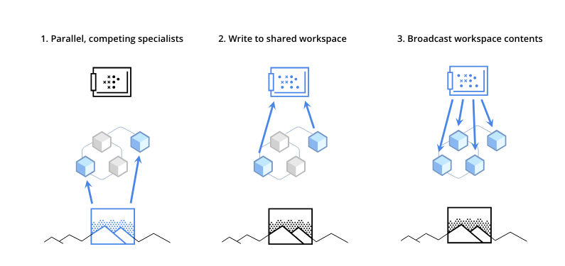
By centralizing communication this way, the model mimics how a human brain might focus only on the most relevant information at any given time. It mimics a sort of “cognitive economy,” where only the most relevant data is processed and shared among modules, filtered through a bottleneck that forces the model to use a highly efficient, reducing-redundancy useful representation, which enhances the overall performance of the system. Moreover, the theory embeds some of the assumptions of the Global Workspace Theory (GWT) of consciousness, which suggests that consciousness arises from the ability of various brain processes to access a shared information platform, the Global Workspace.
Section 2: Higher order assessment and metacognition#
Video 5: Higher order assessment and metacognition#
Submit your feedback#
Show code cell source
# @title Submit your feedback
content_review(f"{feedback_prefix}_Video_5")
Second order model#
Blindsight is a neurological phenomenon where individuals with damage to their primary visual cortex can still respond to visual stimuli without consciously perceiving them. Megan showed you a video of this from a real patient navigating a corridor and successfully avoiding objects that researchers had strategically placed in his way, which the patient navigated successfully.
To study this, we use a simulated dataset that mimics the conditions of blindsight. This dataset contains 400 patterns, equally split between two types:
Random noise patterns consist of low activations ranging between 0.0 and 0.02.
Designed stimulus patterns - each pattern includes one unit that shows a higher activation level, varying between 0.0 and 1.0.
This dataset allows us to test hypotheses concerning how sensory processing and network responses adapt under different conditions of visual impairment.
We have three main testing scenarios, each designed to alter the signal-to-noise ratio to simulate different levels of visual impairment:
Suprathreshold stimulus condition: here, the network is tested against familiar patterns used during training to assess its response to known stimuli.
Subthreshold stimulus condition: this condition slightly increases the noise level, akin to actual blindsight conditions, testing the network’s capability to discern subtle signals.
Low vision condition: the intensity of stimuli is decreased to evaluate how well the network performs with significantly reduced sensory input.
factor=2

initialize_global()
set_1, _ = create_patterns(0,factor)
set_2, _ = create_patterns(1,factor)
set_3, _ = create_patterns(2,factor)

# Plot
plot_signal_max_and_indicator(set_1.detach().cpu(), "Suprathreshold dataset")
plot_signal_max_and_indicator(set_2.detach().cpu(), "Subthreshold dataset")
plot_signal_max_and_indicator(set_3.detach().cpu(), "Low Vision dataset")
The first-order network model lays the groundwork for our experiments and is structured as follows:
Input layer: consists of 100 units representing either noise or stimulus patterns.
Hidden layer: includes a 40-unit layer tasked with processing the inputs.
Output layer: comprises 100 units where the responses to stimuli are recorded.
Dropout and activation: includes dropout layers to prevent overfitting and a temperature-controlled activation function to fine-tune response sharpness.
The primary aim of the first-order network is to accurately capture and react to the input patterns, setting a baseline for comparison with more complex models.
Coding Exercise 2: Developing a Second-Order Network#
Your task is to expand upon the first-order network by integrating a second-order network that incorporates a metacognitive layer assessing the predictions of the first-order network. This metacognitive layer introduces a wagering mechanism, wherein the network “bets” on its confidence in its predictions.
The first-order network is designed as an autoencoder, a type of neural network trained to reconstruct the input stimulus. The autoencoder consists of an encoder that compresses the input into a latent representation and a decoder that reconstructs the input from this representation.
The second-order network, or metacognitive layer, operates by examining the difference (delta) between the original input and the output generated by the autoencoder. This difference provides insight into the reconstruction error, which is a measure of how accurately the autoencoder has learned to replicate the input data. By evaluating this reconstruction error, the second-order network can make a judgement about the certainty of the first-order network’s predictions.
These are the steps for completion:
Architectural development: grasp the underlying principles of a second-order network and complete the architectural code.
Performance evaluation: visualize training losses and test the model using provided code, assessing its initial performance.
Model fine-tuning: leveraging the provided training function, experiment with fine-tuning the model to enhance its accuracy and efficiency.
The second-order network is structured as a feedforward backpropagation network.
Input layer: comprises a 100-unit comparison matrix. This matrix quantifies the discrepancy between each corresponding pair of input and output units from the first-order network. For example, if an input unit and its corresponding output unit have activations of 0.6 and 0.7, respectively, the comparison unit’s activation would be -0.1. This setup essentially encodes the prediction error of the first-order network’s outputs as an input pattern for the second-order network.
Output layer: consists of two units representing “high” and “low” wagers, indicating the network’s confidence in its predictions. The initial weights for these output units range between 0.0 and 0.1.
Comparator weights: set to 1.0 for connections from the first-order input layer to the comparison matrix, and -1.0 for connections from the first-order output layer. This configuration emphasizes the differential error as a critical input for the second-order decision-making process.
The second-order network’s novel approach uses the error generated by the first-order network as a direct input for making decisions—specifically, wagering on the confidence of its outputs. This methodology reflects a metacognitive layer of processing, akin to evaluating one’s confidence in their answers or predictions.
By exploring these adjustments, you can optimize the network’s functionality, making it a powerful tool for understanding and simulating complex cognitive phenomena like blindsight.
class SecondOrderNetwork(nn.Module):
    def __init__(self, use_gelu):
        super(SecondOrderNetwork, self).__init__()
        # Define a linear layer for comparing the difference between input and output of the first-order network
        self.comparison_layer = nn.Linear(100, 100)

        # Linear layer for determining wagers, mapping from 100 features to a single output
        self.wager = nn.Linear(100, 1)

        # Dropout layer to prevent overfitting by randomly setting input units to 0 with a probability of 0.5 during training
        self.dropout = nn.Dropout(0.5)

        # Select activation function based on the `use_gelu` flag
        self.activation = torch.relu

        # Additional activation functions for potential use in network operations
        self.sigmoid = torch.sigmoid

        self.softmax = nn.Softmax()

        # Initialize the weights of the network
        self._init_weights()

    def _init_weights(self):
        # Uniformly initialize weights for the comparison and wager layers
        init.uniform_(self.comparison_layer.weight, -1.0, 1.0)
        init.uniform_(self.wager.weight, 0.0, 0.1)

    def _init_weights(self):
        # Uniformly initialize weights for the comparison and wager layers
        init.uniform_(self.comparison_layer.weight, -1.0, 1.0)
        init.uniform_(self.wager.weight, 0.0, 0.1)

    def forward(self, first_order_input, first_order_output):
        ############################################################
        # Fill in the wager value
        # Applying dropout and sigmoid activation to the output of the wager layer
        raise NotImplementedError("Student exercise")
        ############################################################

        # Calculate the difference between the first-order input and output
        comparison_matrix = first_order_input - first_order_output

        #Another option is to directly calculate the per unit MSE to use as input for the comparator matrix
        #comparison_matrix = nn.MSELoss(reduction='none')(first_order_output, first_order_input)

        # Pass the difference through the comparison layer and apply the chosen activation function
        comparison_out=self.dropout(self.activation(self.comparison_layer(comparison_matrix)))

        # Calculate the wager value, applying dropout and sigmoid activation to the output of the wager layer
        wager = ...

        return wager
Submit your feedback#
Show code cell source
# @title Submit your feedback
content_review(f"{feedback_prefix}_Second_Order_Network")
hidden=40
factor=2
gelu=False
gam=0.98
meta=True
stepsize=25

initialize_global()

# First order network instantiation
first_order_network = FirstOrderNetwork(hidden, factor, gelu).to(device)
def pre_train(first_order_network, second_order_network, criterion_1,  criterion_2, optimizer_1, optimizer_2, scheduler_1, scheduler_2, factor, meta):
    """
    Conducts pre-training for first-order and second-order networks.

    Parameters:
    - first_order_network (torch.nn.Module): Network for basic input-output mapping.
    - second_order_network (torch.nn.Module): Network for decision-making based on the first network's output.
    - criterion_1, criterion_2 (torch.nn): Loss functions for the respective networks.
    - optimizer_1, optimizer_2 (torch.optim): Optimizers for the respective networks.
    - scheduler_1, scheduler_2 (torch.optim.lr_scheduler): Schedulers for learning rate adjustment.
    - factor (float): Parameter influencing data augmentation or pattern generation.
    - meta (bool): Flag indicating the use of meta-learning strategies.

    Returns:
    Tuple containing updated networks and epoch-wise loss records.

    """
    def get_num_args(func):
      return func.__code__.co_argcount

    max_values_output_first_order = []
    max_indices_output_first_order = []
    max_values_patterns_tensor = []
    max_indices_patterns_tensor = []

    epoch_1_order = np.zeros(n_epochs)
    epoch_2_order = np.zeros(n_epochs)

    for epoch in range(n_epochs):
        # Generate training patterns and targets for each epoch
        patterns_tensor, stim_present_tensor, stim_absent_tensor, order_2_tensor = generate_patterns(patterns_number, num_units,factor, 0)

        # Forward pass through the first-order network
        hidden_representation , output_first_order = first_order_network(patterns_tensor)

        patterns_tensor=patterns_tensor.requires_grad_(True)
        output_first_order=output_first_order.requires_grad_(True)

        # Get max values and indices for output_first_order
        max_vals_out, max_inds_out = torch.max(output_first_order[100:], dim=1)
        max_inds_out[max_vals_out == 0] = 0
        max_values_output_first_order.append(max_vals_out.tolist())
        max_indices_output_first_order.append(max_inds_out.tolist())

        # Get max values and indices for patterns_tensor
        max_vals_pat, max_inds_pat = torch.max(patterns_tensor[100:], dim=1)
        max_inds_pat[max_vals_pat == 0] = 0
        max_values_patterns_tensor.append(max_vals_pat.tolist())
        max_indices_patterns_tensor.append(max_inds_pat.tolist())

        optimizer_1.zero_grad()

        # Conditionally execute the second-order network pass and related operations
        if meta:

            # Forward pass through the second-order network with inputs from the first-order network
            output_second_order = second_order_network(patterns_tensor, output_first_order)

            # Calculate the loss for the second-order network (wagering decision based on comparison)
            loss_2 = criterion_2(output_second_order.squeeze(), order_2_tensor[:, 0])

            optimizer_2.zero_grad()


            # Backpropagate the second-order network's loss
            loss_2.backward(retain_graph=True)  # Allows further backpropagation for loss_1 after loss_2

            # Update second-order network weights
            optimizer_2.step()

            scheduler_2.step()

            epoch_2_order[epoch] = loss_2.item()
        else:
            # Skip computations for the second-order network
            with torch.no_grad():
                # Potentially forward pass through the second-order network without tracking gradients
                output_second_order = second_order_network(patterns_tensor, output_first_order)

        # Calculate the loss for the first-order network (accuracy of stimulus representation)

        num_args = get_num_args(criterion_1)

        if num_args == 2:
          loss_1 = criterion_1(  output_first_order , stim_present_tensor )
        else:
          W = first_order_network.state_dict()['fc1.weight']
          loss_1 = criterion_1( W, stim_present_tensor.view(-1, 100), output_first_order,
                             hidden_representation, lam )

        # Backpropagate the first-order network's loss
        loss_1.backward()

        # Update first-order network weights
        optimizer_1.step()

        # Reset first-order optimizer gradients to zero for the next iteration

        # Update the first-order scheduler
        scheduler_1.step()

        epoch_1_order[epoch] = loss_1.item()
        #epoch_1_order[epoch] = loss_location.item()

    return first_order_network, second_order_network, epoch_1_order, epoch_2_order , (max_values_output_first_order[-1],
            max_indices_output_first_order[-1],
            max_values_patterns_tensor[-1],
            max_indices_patterns_tensor[-1])

# Define the architecture, optimizers, loss functions, and schedulers for pre training
seeds=15

results_seed=[]
discrimination_seed=[]

# Hyperparameters
optimizer="ADAMAX"
hidden=40
factor=2
gelu=False
gam=0.98
meta=True
stepsize=25

for i in range(seeds):
  print(f"Seed {i}")

  # Compare your results with the patterns generate below
  initialize_global()

  # Prepare networks, loss functions, optimizers, and schedulers for pre-training
  first_order_network, second_order_network, criterion_1, criterion_2, optimizer_1, optimizer_2, scheduler_1, scheduler_2 = prepare_pre_training(hidden, factor, gelu, stepsize, gam)

  # Conduct pre-training for both the first-order and second-order networks
  first_order_network_pre, second_order_network_pre, epoch_1_order, epoch_2_order , max_value_indices = pre_train(first_order_network, second_order_network, criterion_1,  criterion_2, optimizer_1, optimizer_2, scheduler_1, scheduler_2, factor, meta)

  # Plot the training progress of both networks to visualize performance and learning trends
  pre_train_plots(epoch_1_order, epoch_2_order, f"1st & 2nd Order Networks - Seed {i}" , max_value_indices )

  # Configuration step for the main training phase or evaluation
  testing_patterns, n_samples = get_test_patterns(factor)

  # Function to test the model using the configured testing patterns
  first_order_network_pre.eval()
  second_order_network_pre.eval()
  f1_scores_wager, mse_losses_indices , mse_losses_values , discrimination_performances, results_for_plotting = testing(testing_patterns, n_samples, first_order_network_pre, second_order_network_pre,factor)
  results_seed.append(results_for_plotting)
  discrimination_seed.append(discrimination_performances)

plot_testing(results_seed, discrimination_seed, seeds, "Test Results")
Discussion point#
Let’s dive into the outcomes!
Did you notice any variations between the two models?
Can you explain how these differences influenced the performance?
What role does a second-order network play, and in which situations would it be more effective?
Submit your feedback#
Show code cell source
# @title Submit your feedback
content_review(f"{feedback_prefix}_Discussion_Point_Second_Order_Network")
Video 6: Second Order Network#
Submit your feedback#
Show code cell source
# @title Submit your feedback
content_review(f"{feedback_prefix}_Video_6")
Higher Order State Space (HOSS) model#
Next, Steve is going to tell us about the higher order state space model of consciousness, including the computational and neurological underpinnings that differentiate conscious from unconscious perception.
Video 7: Higher-Order State Spaces#
Submit your feedback#
Show code cell source
# @title Submit your feedback
content_review(f"{feedback_prefix}_Video_7")
In this section, we’ll merge ideas from earlier discussions to present a fresh perspective on how conscious awareness might arise in neural systems. This view comes from higher-order theory, which suggests that consciousness stems from the ability to monitor basic, or first-order, information processing activities, instead of merely broadcasting information globally. This concept emphasizes the need for a comprehensive monitor that oversees various first-order processes (like GWT). It extends the idea of the role of a second-order network, which helps us understand phenomena like blindsight.
To analyze how our brains handle and update perceptions, we’ll use a Bayesian framework. This framework helps us evaluate how we perceive reality based on the information we receive. For example, if you hear rustling leaves, your brain calculates the likelihood of it being caused by the wind versus an animal. This calculation involves updating what we initially guess (our prior belief) with new evidence (observed data), resulting in a new, more informed belief (posterior probability).
The function below calculates these updated beliefs and uses Kullback-Leibler (KL) divergence to quantify how much the new information changes our understanding. The KL divergence is a way of measuring the ‘distance’ between the initial belief and your updated belief. In essence, it’s measuring how much you have to change your mind given new evidence.
We base our analysis on a flat, or single-layer, Bayesian network model. This model directly connects our sensory inputs with our perceptual states, simplifying the complex interactions in our brain into a more manageable form. By stripping away the complexities of multi-layered networks, we focus purely on how direct observations impact our consciousness. This simplified approach helps us to better understand the intricate dance between perception and awareness in our neural systems.
def HOSS_evaluate_flat(X, mu, Sigma, Wprior):
    """
    Perform inference on a 2D Bayes net for asymmetric inference on presence vs. absence.

    Parameters:
    X - Observed data
    mu - Means for each perceptual state
    Sigma - Covariance matrix
    Wprior - Prior probabilities of perceptual states

    #Returns:
    post_W - Posterior probabilities of perceptual states
    KL_W - Kullback-Leibler divergence from posterior to prior
    """
    # Prior on perceptual states W
    p_W = Wprior

    # Compute likelihood of observed X for each possible W (P(X|W))
    log_lik_X_W = np.array([np.log(multivariate_normal.pdf(X, mean=mu[m], cov=Sigma)) for m in range(mu.shape[0])])

    # Renormalize to get P(X|W)
    log_p_X_W = log_lik_X_W - logsumexp(log_lik_X_W)

    # Posterior over W (P(W|X=x))
    log_post_W = log_p_X_W + np.log(p_W)
    log_post_W = log_post_W - logsumexp(log_post_W)  # Normalize
    post_W = np.exp(log_post_W)

    # KL divergences
    KL_W = np.sum(post_W * (np.log(post_W) - np.log(p_W)))

    return post_W, KL_W
Defining our Stimulus Space#
The model we are using is grounded in classical Signal Detection Theory (SDT). SDT is a special case of a Bayesian generative model, in which an arbitrary evidence value is drawn from an unknown distribution. The task of the observer is to infer which distribution this evidence came from.
In SDT, an observer receives a piece of evidence (this could be any sensory input, like a sound, a light signal, or a statistical data point). The evidence comes from one of several potential distributions. Each distribution represents a different state of the world. For instance, one distribution might represent the presence of a signal (like a beep), while another might represent just noise. The observer uses Bayesian inference to assess the probability that the received evidence came from one distribution or another. This involves updating their beliefs (probabilities) based on the new evidence. Based on the probabilities calculated through Bayesian inference, the observer decides which distribution most likely produced the evidence.
Let’s now imagine we have two categories, A and B - for instance, left- and right-tilted visual stimuli. The sensory evidence can be written as 2D vector, where the first element is evidence for A, and the second element evidence for B:
# Creating the array X with strong evidence for A and weak evidence for B
X = np.array([1.5, 0])
The origin (0,0) represents low activation of both features, consistent with no stimulus (or noise) being presented. Comparing how the model handles inference on stimulus presence vs. absence - detecting, vs. not detecting a stimulus - allows us to capture the classical conscious vs. unconscious contrast in consciousness science.
Let’s start by creating our space, and placing three Gaussian distributions on the space that represent the likelihood of observing a pair of features given each of three stimulus classes:
leftward tilt (\(w_1\))
rightward tilt (\(w_2\))
noise/nothing (\(w_0\))
By setting up this model, we aim to simulate and analyze how an observer infers the presence or absence of a stimulus. When the observer detects a stimulus, the inference process would lean towards either the leftward or rightward tilt, depending on which Gaussian (\(w_1\) or \(w_2\)) the observed data points are closer to in feature space. When the observer fails to detect a stimulus, the inference process would recognize that the data points fall closer to the noise distribution centered at the origin.
# Define the grid
xgrid = np.arange(-4, 6.02, 0.02)
X1, X2 = np.meshgrid(xgrid, xgrid)

# Mean and covariance of the distributions
mu = np.array([[0.5, 0.5], [3.5, 0.5], [0.5, 3.5]])
Sigma = np.array([[1, 0], [0, 1]])

# Plotting
with plt.xkcd():
    fig = plt.figure(figsize=(5, 5))
    ax = fig.add_subplot(111)

    # Colors and labels according to the specification
    colors = ['green', 'blue', 'red']
    labels = ['no stimulus', 'left tilt', 'right tilt']

    for i, (color, label) in enumerate(zip(colors, labels)):
        p = multivariate_normal.pdf(np.dstack((X1, X2)), mean=mu[i], cov=Sigma)
        ax.contour(X1, X2, p.reshape(X1.shape), colors=color, alpha=0.5)

    # Create custom legends
    legend_elements = [Patch(facecolor=color, edgecolor='k', label=label) for color, label in zip(colors, labels)]
    ax.legend(handles=legend_elements, loc='upper right')

    # Reverse the X1 axis
    ax.set_xlim([-.5, 6])
    ax.set_ylim([-0.5, 6])
    ax.set_xlabel('evidence for left tilt')
    ax.set_ylabel('evidence for right tilt')
    ax.set_title('2D SDT')

    plt.show()
Let’s measure the evidence for each of the three classes at each point in the space. We’ll then use this evidence to calculate the posterior probability of each class given the evidence. This calculation will help us understand how the observer’s beliefs change based on the sensory data they receive.
coords = np.linspace(-.5, 6.5, 27)
left, right = np.meshgrid(coords, coords)
Xs = np.stack([left.ravel(), right.ravel()], axis=1)
# Define the input parameters

mu = np.array([[0.5, 0.5], [3.5, 0.5], [0.5, 3.5]])
Sigma = np.array([[1, 0], [0, 1]])
Wprior = np.array([1/3, 1/3, 1/3])  # flat priors

cmap = plt.cm.colors.ListedColormap(['green', 'blue', 'red'])

# Under this configuration, the posterior probabilities and KL divergences are calculated
most_likely_class = []
KL_Ws = []
for i in range(Xs.shape[0]):
    post_w, KL_W = HOSS_evaluate_flat(Xs[i, :], mu, Sigma, Wprior)
    most_likely_class.append(np.argmax(post_w))
    KL_Ws.append(KL_W)

most_likely_class = np.array(most_likely_class).reshape(left.shape)
KL_Ws = np.array(KL_Ws).reshape(left.shape)

with plt.xkcd():
    fig, ax = plt.subplots(ncols=2, figsize=(8, 6), layout='compressed')

    im = ax[0].imshow(most_likely_class, extent=[coords[0], coords[-1], coords[-1], coords[0]], cmap=cmap)
    ax[0].set_ylim([coords[0], coords[-1]])
    ax[0].set_title("Most likely class")
    cb = plt.colorbar(im, ax=ax[0], ticks=[0, 1, 2])
    cb.ax.set_yticklabels(['none', 'left', 'right'])
    ax[0].set_xlabel('left tilt evidence')
    ax[0].set_ylabel('right tilt evidence')

    im = ax[1].imshow(KL_Ws, extent=[coords[0], coords[-1], coords[-1], coords[0]])
    ax[1].set_ylim([coords[0], coords[-1]])
    ax[1].set_title("KL divergence")
    plt.colorbar(im, ax=ax[1])
    ax[1].set_xlabel('left tilt evidence')
    ax[1].set_ylabel('right tilt evidence')
The model partitions the stimuli in the expected way. KL divergence is higher further away from the boundaries, as measuring stimuli far away from the boundaries makes the model rapidly update its beliefs. This is because the model is more certain about the stimuli’s class when they are far from the boundaries.
Add in higher-order node for global detection#
So far, our model has been straightforward, or flat, where each perceptual state (like leftward tilt, rightward tilt, or no stimulus) is treated separately. However, real-life perception often requires more complex judgments about the presence or absence of any stimulus, not just identifying specific types. This is where a higher-order node comes into play.
Introducing the “A” Level:#
Think of the “A” level as a kind of overseer or monitor that watches over the lower-level states (\(w_1\), \(w_2\), etc.). This higher-order node isn’t concerned with the specific content of the stimulus (like which direction something is tilting) but rather with whether there’s any significant stimulus at all versus just noise. It takes inputs from the same data (pairs of \(X\)’s), but it adds a layer of awareness. It evaluates whether the data points suggest any meaningful content or if they’re likely just random noise.
The system can now answer questions on two levels:
the content level (W-level)
the awareness or presence of any content (A-level)
The output from the A-level, denoted as post_A, represents the posterior probability that there is any relevant content as opposed to mere noise. To make this work, we also need to set priors (initial guesses before seeing the data) at both the W-level (content) and A-level (awareness). This helps the model start with a baseline expectation about the likelihood of encountering various stimuli or noise.
In the next sections, we will illustrate the operation of a higher-order state space (HOSS) for monitoring first-order information processing. This model, with its higher-order node, mimics human perceptual processing where not every sensory input leads to awareness.

Model inference#
We denote an observation \(\mathbf{X}\) as a pair of features \((X_1, X_2)\), where \(X_1\) and \(X_2\) are the evidence for the presence of two different stimuli. The observer’s task is to infer which of three possible stimuli \(W \in [w_0, w_1, w_2]\) generated the observation. Each stimulus \(W\) is associated with a Gaussian distribution in the feature space:
where \(\mathbf{\mu_W}\) is the mean of each Gaussian, and \(\mathbf{\Sigma}\) is the covariance matrix.
At a higher level, the observer also needs to infer the presence of any stimulus, regardless of its specific type. This is done by calculating the posterior probability of the awareness state \(A\) given the observation:
where:
\(A\) is the awareness state, a two-dimensional binary variable, with \(A_0\) representing no stimulus and \(A_1\) representing the presence of a stimulus
\(P(A)\) is the prior probability of each awareness state
\(P(W|A)\) is the likelihood of each world state given the awareness state. This is 0 for the no stimulus state and \(p(W)\) for the stimulus present states.
\(P(X=x|W)\) is the likelihood of the observation given each world state.
Finally, the observer can calculate the posterior probability of each stimulus class given the observation and the awareness state:
With these equations, we’re ready to simulate the observer’s inference process and explore how the model behaves under different conditions.
Coding exercise#
def HOSS_evaluate(X, mu, Sigma, Aprior, Wprior):
    """

    Inference on 2D Bayes net for asymmetric inference on presence vs. absence.
    """

    #################################################
    ## TODO for students: fill in the missing variables ##
    # Fill out function and remove
    raise NotImplementedError("Student exercise: fill in the missing variables")
    #################################################

    # Initialise variables and conditional prob tables
    p_A = np.array([1 - Aprior, Aprior])  # prior on awareness state A
    p_W_a1 = np.append(0, Wprior)  # likelihood of world states W given aware, first entry is absence
    p_W_a0 = np.append(1, np.zeros(len(Wprior)))  # likelihood of world states W given unaware, first entry is absence
    p_W = (p_W_a1 + p_W_a0) / 2  # prior on W marginalising over A (for KL)

    # Compute likelihood of observed X for each possible W (P(X|mu_w, Sigma))
    lik_X_W = np.array([multivariate_normal.pdf(X, mean=mu_i, cov=Sigma) for mu_i in mu])
    p_X_W = lik_X_W / lik_X_W.sum()  # normalise to get P(X|W)

    # Combine with likelihood of each world state w given awareness state A
    lik_W_A = np.vstack((p_X_W * p_W_a0 * p_A[0], p_X_W * p_W_a1 * p_A[1]))
    post_A = ...  # sum over W
    post_A = post_A / post_A.sum()  # normalise

    # Posterior over W (P(W|X=x) marginalising over A)
    post_W = ...  # sum over A
    post_W = post_W / post_W.sum()  # normalise

    # KL divergences
    KL_W = (post_W * np.log(post_W / p_W)).sum()
    KL_A = (post_A * np.log(post_A / p_A)).sum()

    return post_W, post_A, KL_W, KL_A
Submit your feedback#
Show code cell source
# @title Submit your feedback
content_review(f"{feedback_prefix}_Hoss")
Now that we’ve coded our multi-level model, we’re ready to evaluate it! We first set the prior on presence (vs. absence), and then set the priors on \(w_1\) vs. \(w_2\), and the model takes care of the rest.
We’ll evaluate the model on the edge between the leftward stimulus \(w_1\) and the absence of a stimulus \(w_0\). This edge case is particularly interesting because it’s where the model is most uncertain about the presence of a stimulus.
# Define the input parameters for this specific example
X = np.array([2, 0.5])  # Input observed features
Wprior = np.array([0.5, 0.5])  # Prior probabilities of stimuli
Aprior = 0.5  # Prior probability of being aware

# Call the HOSS_evaluate function with the specified parameters
post_W, post_A, KL_W, KL_A = HOSS_evaluate(X, mu, Sigma, Aprior, Wprior)

# Print the posterior probabilities
print(f"Posterior probabilities at W level: {post_W}")
print(f"Posterior probability at awareness at A level: {post_A[1]}")
We notice two things:
The model is fairly certain that the stimulus is absent; the probability of awareness is < 0.5.
The model nevertheless assigns much higher probability to the presence of the leftward stimulus \(w_1\) than to the rightward stimulus \(w_2\).
This captures the essence of a phenomenon like blindsight: there can be positive discrimination between different stimuli even when the observer is not consciously aware of the stimulus. Let’s look at how the awareness signal changes as the evidence changes.
coords = np.linspace(-.5, 6.5, 27)
left, right = np.meshgrid(coords, coords)
Xs = np.stack([left.ravel(), right.ravel()], axis=1)
# Define the input parameters

mu = np.array([[0.5, 0.5], [3.5, 0.5], [0.5, 3.5]])
Sigma = np.array([[1, 0], [0, 1]])
Wprior = np.array([.5, .5])  # flat priors

# Under this configuration, the posterior probabilities and KL divergences are calculated
rightwards = []
awareness = []
for i in range(Xs.shape[0]):
    post_W, post_A, KL_W, KL_A = HOSS_evaluate(Xs[i, :], mu, Sigma, Aprior, Wprior)
    rightwards.append(post_W[2] / (post_W[1] + post_W[2]))
    awareness.append(post_A[1])

rightwards = np.array(rightwards).reshape(left.shape)
awareness = np.array(awareness).reshape(left.shape)

with plt.xkcd():
    fig, ax = plt.subplots(ncols=2, figsize=(8, 6), layout='compressed')


    im = ax[0].imshow(awareness, extent=[coords[0], coords[-1], coords[-1], coords[0]])
    ax[0].set_ylim([coords[0], coords[-1]])
    ax[0].set_title("P(awareness)")
    cb = plt.colorbar(im, ax=ax[0], ticks=[0, 1, 2])
    ax[0].set_xlabel('left tilt evidence')
    ax[0].set_ylabel('right tilt evidence')

    im = ax[1].imshow(rightwards, extent=[coords[0], coords[-1], coords[-1], coords[0]])
    ax[1].set_ylim([coords[0], coords[-1]])
    ax[1].set_title("P(rightwards)")
    plt.colorbar(im, ax=ax[1])
    ax[1].set_xlabel('left tilt evidence')
    ax[1].set_ylabel('right tilt evidence')
Notice that in the bottom left, the probability of awareness is low, even as the evidence for leftward or rightward tilt can be high.
We have included some further details on the notion of ignition. Please feel free to toggle the switch below to learn more. If you’re running low on time, then please feel free to run the cell below and come back to this section. The outro video will also cover the broad overview of this concept.
Simulate Ignition (assymetry vs symmetry)
The HOSS architecture is designed to detect whether something is there or not. When it detects something, it ends up making more prediction errors in its predictions compared to when it detects nothing. These prediction errors are tracked using a method called Kullback-Leibler (KL) divergence, particularly at a certain level within the model known as the W level.
This increase in prediction errors when something is detected is similar to what happens in the human brain, a phenomenon known as global ignition responses. These are big surges in brain activity that happen when we become conscious of something. Research like that conducted by Del Cul et al. (2007) and Dehaene and Changeux (2011) support this concept, linking it to the global workspace model. This model describes consciousness as the sharing of information across different parts of the brain.
In our model, we simulate this by adjusting the intensity of the stimulus and observing how the prediction errors vary in the model. Under a theory called predictive coding, which describes how the brain processes information, KL divergence acts like a marker for neural activity, making it a good stand-in for studying brain-like responses.
We then classify these prediction errors based on whether the model recognizes a stimulus as “seen” or “unseen.” If the model has a response indicating “seen,” it shows more activity than when it indicates “unseen.” This is what we refer to as ignition — more activity for “seen” stimuli.
However, it’s crucial to understand that in the HOSS model, these ignition-like responses don’t directly cause the global sharing of information in the network. Rather, they are secondary effects or byproducts of other calculations happening within the network. Essentially, these bursts of activity are outcomes of deeper processes in the network, not the direct mechanisms for distributing information throughout the system.
# Experiment parameters
mu = np.array([[0.5, 0.5], [3.5, 0.5], [0.5, 3.5]])
Nsubjects = 30
Ntrials = 600
cond = np.concatenate((np.ones(Ntrials//3), np.ones(Ntrials//3)*2, np.ones(Ntrials//3)*3))
Wprior = [0.5, 0.5]
Aprior = 0.5

# Sensory precision values
gamma = np.linspace(0.1, 10, 6)

# Initialize lists for results
all_KL_w_yes = []
sem_KL_w_yes = []
all_KL_w_no = []
sem_KL_w_no = []
all_KL_A_yes = []
sem_KL_A_yes = []
all_KL_A_no = []
sem_KL_A_no = []
all_prob_y = []

for y in tqdm(gamma, desc='Processing gammas'):
    Sigma = np.diag([1./np.sqrt(y)]*2)
    mean_KL_w = np.zeros((Nsubjects, 4))
    mean_KL_A = np.zeros((Nsubjects, 4))
    prob_y = np.zeros(Nsubjects)

    for s in tqdm(range(Nsubjects), desc=f'Subjects for gamma={y}', leave=False):
        KL_w = np.zeros(len(cond))
        KL_A = np.zeros(len(cond))
        posteriorAware = np.zeros(len(cond))

        # Generate sensory samples
        X = np.array([multivariate_normal.rvs(mean=mu[int(c)-1, :], cov=Sigma) for c in cond])

        # Model inversion for each trial
        for i, x in enumerate(X):
            post_w, post_A, KL_w[i], KL_A[i] = HOSS_evaluate(x, mu, Sigma, Aprior, Wprior)
            posteriorAware[i] = post_A[1]  # Assuming post_A is a tuple with awareness probability at index 1

        binaryAware = posteriorAware > 0.5
        for i in range(4):
            conditions = [(cond == 1), (cond != 1), (cond == 1), (cond != 1)]
            aware_conditions = [(binaryAware == 0), (binaryAware == 0), (binaryAware == 1), (binaryAware == 1)]
            mean_KL_w[s, i] = np.mean(KL_w[np.logical_and(aware_conditions[i], conditions[i])])
            mean_KL_A[s, i] = np.mean(KL_A[np.logical_and(aware_conditions[i], conditions[i])])

        prob_y[s] = np.mean(binaryAware[cond != 1])

    # Aggregate results across subjects
    all_KL_w_yes.append(np.nanmean(mean_KL_w[:, 2:4].flatten()))
    sem_KL_w_yes.append(np.nanstd(mean_KL_w[:, 2:4].flatten()) / np.sqrt(Nsubjects))
    all_KL_w_no.append(np.nanmean(mean_KL_w[:, :2].flatten()))
    sem_KL_w_no.append(np.nanstd(mean_KL_w[:, :2].flatten()) / np.sqrt(Nsubjects))
    all_KL_A_yes.append(np.nanmean(mean_KL_A[:, 2:4].flatten()))
    sem_KL_A_yes.append(np.nanstd(mean_KL_A[:, 2:4].flatten()) / np.sqrt(Nsubjects))
    all_KL_A_no.append(np.nanmean(mean_KL_A[:, :2].flatten()))
    sem_KL_A_no.append(np.nanstd(mean_KL_A[:, :2].flatten()) / np.sqrt(Nsubjects))
    all_prob_y.append(np.nanmean(prob_y))

with plt.xkcd():

    # Create figure
    plt.figure(figsize=(10, 5))

    # First subplot: Probability of reporting "seen" for w_1 or w_2
    plt.subplot(1, 3, 1)
    plt.plot(gamma, all_prob_y, linewidth=2)
    plt.xlabel('Stimulus strength')
    plt.ylabel('Prob. report "seen" for w_1 or w_2')
    plt.xticks(fontsize=14)
    plt.yticks(fontsize=14)
    plt.box(False)

    # Second subplot: K-L divergence, perceptual states
    plt.subplot(1, 3, 2)
    plt.errorbar(gamma, all_KL_w_yes, yerr=sem_KL_w_yes, linewidth=2, label='Seen')
    plt.errorbar(gamma, all_KL_w_no, yerr=sem_KL_w_no, linewidth=2, label='Unseen')
    plt.legend(frameon=False)
    plt.xlabel('Stimulus strength')
    plt.ylabel('KL-divergence, perceptual states')
    plt.xticks(fontsize=14)
    plt.yticks(fontsize=14)
    plt.box(False)

    # Third subplot: K-L divergence, awareness state
    plt.subplot(1, 3, 3)
    plt.errorbar(gamma, all_KL_A_yes, yerr=sem_KL_A_yes, linewidth=2, label='Seen')
    plt.errorbar(gamma, all_KL_A_no, yerr=sem_KL_A_no, linewidth=2, label='Unseen')
    plt.legend(frameon=False)
    plt.xlabel('Stimulus strength')
    plt.ylabel('KL-divergence, awareness state')
    plt.xticks(fontsize=14)
    plt.yticks(fontsize=14)
    plt.box(False)

    # Adjust layout and display the figure
    plt.tight_layout()
    plt.show()
Submit your feedback#
Show code cell source
# @title Submit your feedback
content_review(f"{feedback_prefix}_Ignition")
Discussion point#
What do you think is the main takeaway on the distinction between the Global Workspace model and the HOSS on ignition?
Now, Steve will give us a brief recap about how the greater prediction error in seen trials reveals the asymmetry in model architecture and its impact on understanding neural signatures of consciousness, contrasting the classical global workspace view with the higher order state view.
Submit your feedback#
Show code cell source
# @title Submit your feedback
content_review(f"{feedback_prefix}_Discussion_Point_HOSS")
Video 8: Outro - Ignition#
Submit your feedback#
Show code cell source
# @title Submit your feedback
content_review(f"{feedback_prefix}_Video_8")
The Big Picture#
Hakwan will now discuss the critical aspects and limitations of current consciousness studies, addressing the challenges in distinguishing theories of consciousness from those merely describing general brain functions. Join us in the next two videos where we wrap up some of the big ideas and try to put them in context for you!
Video 9: Final Thoughts#
Submit your feedback#
Show code cell source
# @title Submit your feedback
content_review(f"{feedback_prefix}_Video_9")
Congrats! You’ve made it to the end of this tutorial. Let’s wrap up.
Video 10: Final Thoughts#
Submit your feedback#
Show code cell source
# @title Submit your feedback
content_review(f"{feedback_prefix}_Video_10")
Tutorial 3 today contains some bonus material based on extensions of what we’ve covered today. There, you’ll find some optional coding & discussion bonus content! Feel free to bookmark and come back to it whenever you are ready.
For the moment, let’s switch to our second topic on the day, arguably one of the most important topics we’ve covered so far: Ethics.