Tutorial 2: Normalization

Tutorial 2: Normalization#

Week 1, Day 5: Microcircuits

By Neuromatch Academy

Content creators: Alish Dipani, Xaq Pitkow

Content reviewers: Yizhou Chen, RyeongKyung Yoon, Ruiyi Zhang, Lily Chamakura, Hlib Solodzhuk, Patrick Mineault

Production editors: Konstantine Tsafatinos, Ella Batty, Spiros Chavlis, Samuele Bolotta, Hlib Solodzhuk

Tutorial Objectives#

Estimated timing of tutorial: 50 minutes

In this tutorial, you will learn about the microcircuit element of normalization, which is a prominent computation in brains and machines. You will see different types of normalization, how to implement them, and observe some of its benefits for generalization.

Tutorial Learning Objectives

Understand how nonlinearities may be universal function approximators, but not all functions are simple to learn.
Implement a family of normalization mechanisms.
Demonstrate how normalization helps in learning and information transmission.

Setup#

Install and import feedback gadget#

Imports#

Figure settings#

Helper functions#

Show code cell source Hide code cell source

# @title Helper functions

# Section 1

# Validation
VAL_X_LOW = 0
VAL_X_HIGH = 1

def store_grads(model, grads_mat):
  """
  Store the gradients of a PyTorch model's layers in a dictionary.

  Inputs:
  - model (torch.nn.Module): The PyTorch model whose gradients will be stored.
  - grads_mat (dict): A dictionary that will store the gradients: the keys correspond to the names of the model's layers, and the values are PyTorch tensors containing the gradients.

  Outputs:
  - grads_mat (dict): The input dictionary `grads_mat` with the updated gradient values.
  """
  for grad_layer_name, grad_layer in model.grad_layers.items():
    if grad_layer_name in grads_mat.keys():
      grads_mat[grad_layer_name] = torch.vstack((
          grads_mat[grad_layer_name],
          grad_layer.grad.detach().cpu()
      ))
    else:
      grads_mat[grad_layer_name] = grad_layer.grad.detach().cpu()
  return grads_mat

def train_sec1(model, train_dataloader, learning_rate, n_epochs, VAL_X_LOW, VAL_X_HIGH, \
          track_grads=False):
  """
  Train a model using the given dataloader, learning rate, and number of epochs.

  Inputs:
  - model (torch.nn.Module): The PyTorch model to be trained.
  - train_dataloader (torch.utils.data.DataLoader): Dataloader for training data.
  - learning_rate (float): The learning rate for the optimizer.
  - n_epochs (int): Number of epochs for training.
  - VAL_X_LOW (float): Lower bound of validation x values.
  - VAL_X_HIGH (float): Upper bound of validation x values.
  - track_grads (bool): Whether to track and store gradients during training.

  Outputs:
  - losses_iter (list of float): List of loss values for each iteration.
  - losses_epoch (list of float): List of loss values for each epoch.
  - training_dynamics_mat (torch.Tensor): Tensor containing the validation errors over training.
  - input_thresholds_tensor (torch.Tensor): Tensor containing the input threshold weights over training.
  - output_weights_tensor (torch.Tensor): Tensor containing the output layer weights over training.
  - gradients_mat (dict, optional): Dictionary containing the gradients if track_grads is True.
  """
  # Training settings
  loss_fn = nn.MSELoss()
  optimizer = torch.optim.SGD(model.parameters(), lr=learning_rate)

  # Train the model
  model.train()
  losses_iter = []
  losses_epoch = []
  # training loss dynamics
  val_x = torch.arange(VAL_X_LOW+1e-2, VAL_X_HIGH, 0.01).unsqueeze(1).to(DEVICE)
  val_y = (1/val_x).to(DEVICE)
  training_dynamics_mat = None
  gradients_mat = {}
  # training weight dynamics
  input_thresholds_tensor = model.input_threshold_weights.cpu().clone().detach()
  output_weights_tensor = model.output_layer.weight.data[0].cpu().clone().detach()
  for epoch in range(n_epochs):
    epoch_loss = 0
    for X_batch, y_batch in train_dataloader:
        X_batch = X_batch.to(DEVICE)
        y_batch = y_batch.to(DEVICE)
        optimizer.zero_grad()
        y_pred = model(X_batch)
        loss = loss_fn(y_pred, y_batch)
        loss.backward()
        optimizer.step()
        with torch.no_grad():
          losses_iter.append(loss.cpu().item())
          epoch_loss += loss.cpu().item()
          if track_grads:
            gradients_mat = store_grads(model, gradients_mat)
    losses_epoch.append(epoch_loss)
    # Store training loss dynamics
    with torch.no_grad():
      val_errors = torch.log(nn.functional.mse_loss(model.predict(val_x), val_y, reduction='none'))
      val_errors = (val_errors.T).cpu()
      if training_dynamics_mat is None:
        training_dynamics_mat = val_errors
      else:
        training_dynamics_mat = torch.vstack((val_errors, training_dynamics_mat))
    # Store training weight dynamics
    epoch_ths = model.input_threshold_weights.cpu().clone().detach()
    epoch_wts = model.output_layer.weight.data[0].cpu().clone().detach()
    input_thresholds_tensor = torch.vstack((input_thresholds_tensor, epoch_ths))
    output_weights_tensor = torch.vstack((output_weights_tensor, epoch_wts))
  if track_grads:
    return losses_iter, losses_epoch, training_dynamics_mat, \
      input_thresholds_tensor, output_weights_tensor, gradients_mat
  else:
    return losses_iter, losses_epoch, training_dynamics_mat, \
      input_thresholds_tensor, output_weights_tensor

def evaluate_sec1(model, test_dataloader):
  """
  Evaluate a model using the given dataloader and return the test loss, input values, true values, and predicted values.

  Inputs:
  - model (torch.nn.Module): The PyTorch model to be evaluated.
  - test_dataloader (torch.utils.data.DataLoader): Dataloader for test data.

  Outputs:
  - test_loss (float): The loss on the test dataset.
  - x_all (torch.Tensor): Tensor containing all input values from the test dataset.
  - y_all (torch.Tensor): Tensor containing all true values from the test dataset.
  - y_pred_all (torch.Tensor): Tensor containing all predicted values from the test dataset.
  """
  # evaluate MSE after training
  model.eval()
  test_loss = 0
  x_all = None
  y_all = None
  y_pred_all = None
  with torch.no_grad():
    for X_batch, y_batch in test_dataloader:
      X_batch = X_batch.to(DEVICE)
      y_batch = y_batch.to(DEVICE)
      y_pred = model.predict(X_batch)
      # Store
      if x_all is None:
        x_all = X_batch.flatten().cpu().detach()
      else:
        x_all = torch.concat((x_all, X_batch.flatten().detach()))

      if y_all is None:
        y_all = y_batch.flatten().cpu().detach()
      else:
        y_all = torch.concat((y_all, y_batch.flatten().detach()))

      if y_pred_all is None:
        y_pred_all = y_pred.flatten().cpu().detach()
      else:
        y_pred_all = torch.concat((y_pred_all, y_pred.flatten().detach()))

      # Calculate loss
      loss = nn.functional.mse_loss(y_pred, y_batch)
      test_loss += loss.cpu()
    return test_loss, x_all, y_all, y_pred_all

# Section 2.2

def visualize_images_sec22(data, data_titles, viz_p):
  """
  Visualize pixels in given data arrays.

  Inputs:
  - data (list of numpy.array): List of numpy arrays to visualize.
  - data_titles (list of str): List of titles for each data array.
  - viz_p (int): Number of samples to visualize.

  Outputs:
  - None: Displays a plot of the data arrays.
  """
  with plt.xkcd():
      vmin = np.min([np.min(arr[: viz_p, :]) for arr in data])
      vmax = np.min([np.max(arr[: viz_p, :]) for arr in data])
      cmap = 'gray_r'
      # Plot
      height_ratios = [10, 2, 10] if len(data)==3 else [10, 2, 10, 10]
      figsize = (8, 6) if len(data)==3 else (8, 8)
      fig, axs = plt.subplots(len(data), 1, figsize=figsize, \
                              gridspec_kw={'height_ratios': height_ratios})
      cbar_ax = fig.add_axes([0.98, 0.125, 0.02, 0.75])  # Define position for colorbar
      for i, data_ in enumerate(data):
          sns.heatmap(data_[:viz_p, :].T, cmap=cmap, annot=False, cbar=(i==0), fmt=".2f", annot_kws={"size": 10},
                      ax=axs[i], linewidths=0, linecolor='black', square=True,
                      cbar_ax=None if i else cbar_ax)
          # Use single colorbar for first heatmap
          # Show axes on all sides
          axs[i].spines['top'].set_visible(True)
          axs[i].spines['right'].set_visible(True)
          axs[i].spines['bottom'].set_visible(True)
          axs[i].spines['left'].set_visible(True)
          axs[i].set_xticks([])
          axs[i].set_yticks([])
          axs[i].set_title(data_titles[i])
          axs[i].set_xlabel('')
          axs[i].set_ylabel('')
      # Set common x and y labels
      fig.text(0.5, 0, 'Samples', ha='center', fontsize=15)
      fig.text(0, 0.5, 'Pixel Intensity', va='center', rotation='vertical', fontsize=15)
      plt.subplots_adjust(wspace=5)  # Adjust the horizontal spacing between subplots
      plt.show()

def subsets(arr, k):
  """
  Generate all possible subsets from arr with length k.

  Inputs:
  - arr (numpy.array): 1-D numpy array or list.
  - k (int): Length of the subsets.

  Outputs:
  - subsets (numpy.array): Array of all possible subsets with length k.
  """
  from itertools import combinations
  return np.array(list(combinations(arr, k)))

# Section 2.3

def train_cnns(model, train_dataloader, learning_rate, momentum, n_epochs):
  """
  Train a CNN model using the given dataloader, learning rate, momentum, and number of epochs.

  Inputs:
  - model (torch.nn.Module): The CNN model to be trained.
  - train_dataloader (torch.utils.data.DataLoader): Dataloader for training data.
  - learning_rate (float): The learning rate for the optimizer.
  - momentum (float): The momentum for the optimizer.
  - n_epochs (int): Number of epochs for training.

  Outputs:
  - losses_iter (list of float): List of loss values for each iteration.
  - losses_epoch (list of float): List of loss values for each epoch.
  """
  # Training settings
  loss_fn = nn.CrossEntropyLoss()
  optimizer = torch.optim.SGD(model.parameters(), lr=learning_rate, \
                              momentum=momentum)

  # Train the model
  model.train()
  losses_iter = []
  losses_epoch = []
  # training loss dynamics
  gradients_mat = {}
  # training weight dynamics
  for epoch in tqdm(range(n_epochs)):
    epoch_loss = 0
    for X_batch, y_batch in train_dataloader:
        X_batch = X_batch.to(DEVICE)
        y_batch = y_batch.to(DEVICE)
        optimizer.zero_grad()
        y_pred = model(X_batch)
        loss = loss_fn(y_pred, y_batch)
        loss.backward()
        optimizer.step()
        with torch.no_grad():
          losses_iter.append(loss.cpu().item())
          epoch_loss += loss.cpu().item()
    losses_epoch.append(epoch_loss)
  return losses_iter, losses_epoch

def evaluate_cnns(model, test_dataloader):
  """
  Evaluate a CNN model using the given dataloader and return the test loss and accuracy.

  Inputs:
  - model (torch.nn.Module): The CNN model to be evaluated.
  - test_dataloader (torch.utils.data.DataLoader): Dataloader for test data.

  Outputs:
  - test_loss (float): The loss on the test dataset.
  - accuracy (float): The accuracy on the test dataset.
  """
  model.eval()
  test_loss = 0
  correct = 0
  total = 0
  with torch.no_grad():
    for X_batch, y_batch in test_dataloader:
      X_batch = X_batch.to(DEVICE)
      y_batch = y_batch.to(DEVICE)
      y_pred = model(X_batch).data
      # Calculate loss
      loss = nn.functional.cross_entropy(y_pred, y_batch)
      test_loss += loss.cpu().item()
      # Calculate accuracy
      # the class with the highest energy is what we choose as prediction
      _, predicted = torch.max(y_pred, 1)
      total += y_pred.size(0)
      correct += (predicted == y_batch).sum().item()
  accuracy = 100 * correct / total
  return test_loss, accuracy

def normalize_implemented(x, sigma, p, g):
  """
  Inputs:
  - x(np.ndarray): Input array (n_samples * n_dim)
  - sigma(float): Smoothing factor
  - p(int): p-norm
  - g(int): scaling factor

  Outputs:
  - xnorm (np.ndarray): normalized values.
  """
  # Raise the absolute value of x to the power p
  xp = np.power(np.abs(x), p)
  # Sum the x over the dimensions (n_dim) axis
  xp_sum = np.sum(np.power(np.abs(x), p), axis=1)
  # Correct the dimensions of xp_sum, and taking the average reduces the dimensions
  # Making xp_sum a row vector of shape (1, n_dim)
  xp_sum = np.expand_dims(xp_sum, axis=1)
  # Raise the sum to the power 1/p and add the smoothing factor (sigma)
  denominator = sigma + np.power(xp_sum, 1/p)
  # Scale the input data with a factor of g
  numerator = x*g
  # Calculate normalized x
  xnorm = numerator/denominator
  return xnorm

# Exercise solutions for correct plot output

class ReLUNet(nn.Module):
  """
  ReLUNet architecture
  Structure is as follows:
  y = Σi(ai * ReLU(θi - x))
  """
  # Define the structure of your network
  def __init__(self, n_units):
    """
    Args:
      n_units (int): Number of hidden units

    Returns:
      Nothing
    """
    super(ReLUNet, self).__init__()
    # Create input thresholds
    self.input_threshold_weights = nn.Parameter(torch.abs(torch.randn(n_units)))
    self.non_linearity = nn.ReLU()
    self.output_layer = nn.Linear(n_units, 1)
    nn.init.xavier_normal_(self.output_layer.weight)

  def forward(self, x):
    """
    Args:
      x: torch.Tensor
        Input tensor of size ([1])
    """
    op = self.input_threshold_weights - x #prepare the input to be passed through ReLU
    op = self.non_linearity(op) #apply ReLU
    op = self.output_layer(op) #run through output layer
    return op

  # Choose the most likely label predicted by the network
  def predict(self, x):
    """
    Args:
      x: torch.Tensor
        Input tensor of size ([1])
    """
    output = self.forward(x)
    return output

non_linearities = {
    'ReLU': nn.ReLU(),
    'ReLU6': nn.ReLU6(),
    'SoftPlus': nn.Softplus(),
    'Sigmoid': nn.Sigmoid(),
    'Tanh': nn.Tanh()
}

def HardTanh(x):
  """
  Calculates `tanh` output for the given input data.

  Inputs:
  - x (np.ndarray): input data.

  Outputs:
  - output (np.ndarray): `tanh(x)`.
  """
  min_val = -1
  max_val = 1
  output = np.copy(x)
  output[output>max_val] = max_val
  output[output<min_val] = min_val
  return output

def LeakyHardTanh(x, leak_slope=0.03):
  """
  Calculate `tanh` output for the given input data with the leaky term.

  Inputs:
  - x (np.ndarray): input data.
  - leak_slope (float, default = 0.03): leaky term.

  Outputs:
  - output (np.ndarray): `tanh(x)`.
  """
  output = np.copy(x)
  output = HardTanh(output) + leak_slope*output
  return output

def InverseLeakyHardTanh(y, leak_slope=0.03):
  """
  Calculate input into the `tanh` function with the leaky term for the given output.

  Inputs:
  - y (np.array): output of leaky tanh function.
  - leak_slope (float, default = 0.03): leaky term.

  Outputs:
  - output (np.array): input into leaky tanh function.
  """
  ycopy = np.copy(y)
  output = np.where(
      np.abs(ycopy) >= 1+leak_slope, \
      (ycopy - np.sign(ycopy))/leak_slope, \
      ycopy/(1+leak_slope)
  )
  return output

Set random seed#

Set device (GPU or CPU)#

GPU is not enabled in this notebook. 
If you want to enable it, in the menu under `Runtime` -> 
`Hardware accelerator.` and select `GPU` from the dropdown menu

Section 1: Can ReLUs implement normalization?#

In this section we will explore how feasible it is to estimate a normalization-like function.

Video 1: Introduction#

Submit your feedback#

The general form of normalization is:

\[\hat{x} = \frac{x}{f(||x||)}\]

There are indeed many options for the specific form of the denominator here; still, what we want to highlight is the essential divisive nature of the normalization.

Evidence suggests that normalization provides a useful inductive bias in artificial and natural systems. However, do we need a dedicated computation that implements normalization?

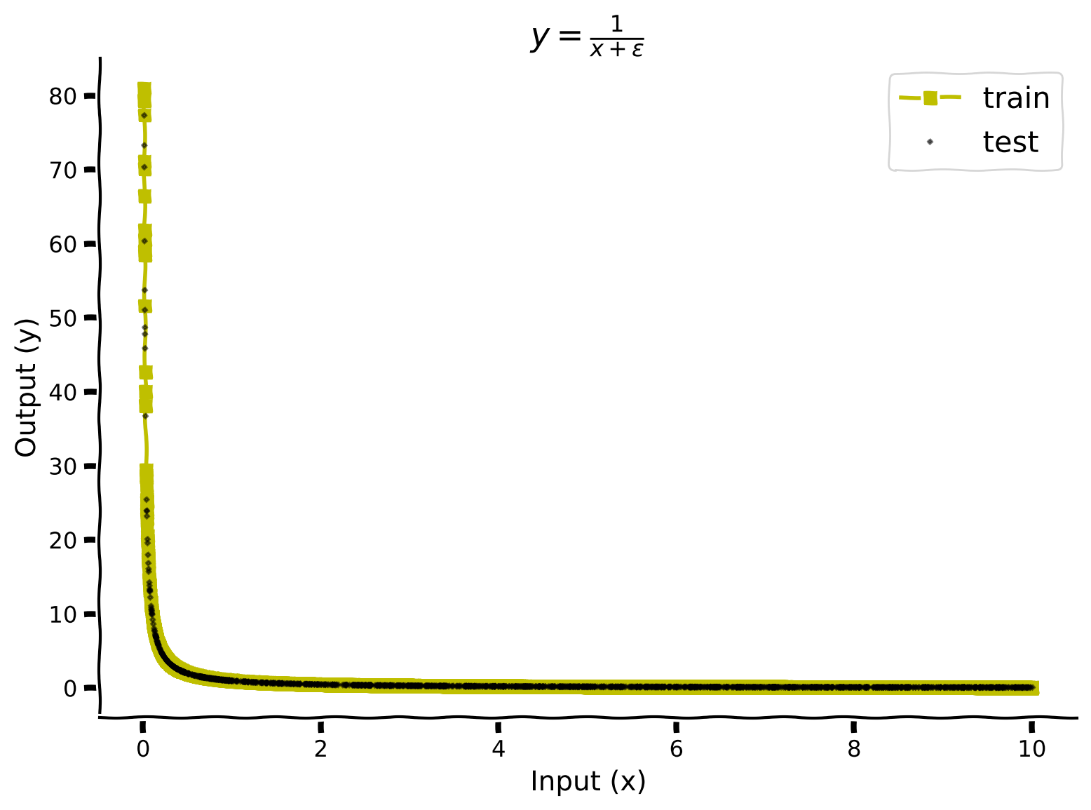
Let’s explore if ReLUs can estimate a normalization-like function. Specifically, we will see if a fully-connected one-layer network can estimate \(y=\frac{1}{x+\epsilon}\) function.

In the cell below, we visualize train and test data.

Generate \(y=\frac{1}{x+\epsilon}\) train and test dataloaders#

\(\epsilon = 0.01\)

Show code cell source Hide code cell source

# @title Generate $y=\frac{1}{x+\epsilon}$ train and test dataloaders
# Target function y = 1/x+ε

# @markdown $\epsilon = 0.01$

N_SAMPLES = 5000
X_LOW = 0
X_HIGH = 10
TRAIN_RATIO = 0.7
EPSILON = 1e-2

range01_ratio = 0.20 # % of samples in the range 0-1
X1 = torch.distributions.uniform.Uniform(X_LOW, 1).rsample(sample_shape=torch.Size([int(N_SAMPLES*range01_ratio), 1]))
X2 = torch.distributions.uniform.Uniform(1, X_HIGH).rsample(sample_shape=torch.Size([int(N_SAMPLES*(1-range01_ratio)), 1]))
X_sec1 = torch.concatenate((X1, X2)) + EPSILON
y_sec1 = 1/X_sec1

class ReLUDataset(Dataset):
  def __init__(self, X, y):
    self.X = X
    self.y = y

  def __len__(self):
    return len(self.y)

  def __getitem__(self, idx):
    X = self.X[idx]
    y = self.y[idx]
    return X, y

dataset_sec1 = ReLUDataset(X_sec1, y_sec1)

# Define the sizes for training and testing sets
train_size = int(TRAIN_RATIO * len(dataset_sec1))
test_size = len(dataset_sec1) - train_size

# Split the dataset into training and testing sets
train_dataset_sec1, test_dataset_sec1 = random_split(dataset_sec1, [train_size, test_size])

# Dataloaders
# Create DataLoader for the training set
train_dataloader_sec1 = DataLoader(train_dataset_sec1, batch_size=len(train_dataset_sec1), shuffle=True)

# Create DataLoader for the testing set
test_dataloader_sec1 = DataLoader(test_dataset_sec1, batch_size=len(test_dataset_sec1), shuffle=False)

train_data = torch.column_stack((train_dataset_sec1.dataset.X[train_dataset_sec1.indices], train_dataset_sec1.dataset.y[train_dataset_sec1.indices]))
sorted_indices = torch.argsort(train_data[:, 0])
train_data_sorted = torch.index_select(train_data, 0, sorted_indices)

with plt.xkcd():
    plt.plot(train_data_sorted[:, 0], train_data_sorted[:, 1], 's-y', label='train')
    plt.plot(test_dataset_sec1.dataset.X[test_dataset_sec1.indices], test_dataset_sec1.dataset.y[test_dataset_sec1.indices], 'Dk', label='test', alpha=0.5, markersize=1.5)
    plt.xlabel('Input (x)')
    plt.ylabel('Output (y)')
    plt.title(r'$y=\frac{1}{x+\epsilon}$')
    plt.legend(prop={'size': 15})
    ax = plt.gca()
    for line in ax.get_lines():
      line.set_path_effects([path_effects.Normal()])
    plt.show()

../../../_images/5c21b5abae4439ba14daef7d8f889baa029267420725410ec80e60ef23d12059.png

Coding Exercise 1: ReLUNet#

Let’s define a simple model having one layer with the equation:

\[\hat{y} = \sum_{i}w_{i} \text{ReLU}(\theta_{i} - x)\]

Here \(\theta_{i}\) is the threshold, and \(w_{i}\) is the slope of neuron \(i\). \(\theta_{i}\) & \(w_{i}\) are learned parameters. Our network has a total of 100 neurons. Complete the forward pass of the model.

###################################################################
## Fill out the following then remove
raise NotImplementedError("Student exercise: complete forward pass.")
###################################################################

class ReLUNet(nn.Module):
  """
  ReLUNet architecture
  The structure is the following:
  y = Σi(wi * ReLU(θi - x))
  """
  # Define the structure of your network
  def __init__(self, n_units):
    """
    Args:
      n_units (int): Number of hidden units

    Returns:
      Nothing
    """
    super(ReLUNet, self).__init__()
    # Create input thresholds
    self.input_threshold_weights = nn.Parameter(torch.abs(torch.randn(n_units)))
    self.non_linearity = nn.ReLU()
    self.output_layer = nn.Linear(n_units, 1)
    nn.init.xavier_normal_(self.output_layer.weight)

  def forward(self, x):
    """
    Args:
      x: torch.Tensor
        Input tensor of size ([1])
    """
    op = ... - ... #prepare the input to be passed through ReLU
    op = self.non_linearity(...) #apply ReLU
    op = ... #run through output layer
    return op

  # Choose the most likely label predicted by the network
  def predict(self, x):
    """
    Args:
      x: torch.Tensor
        Input tensor of size ([1])
    """
    output = self.forward(x)
    return output

Click for solution

Now, let’s train the model and evaluate it.

Training & Evaluating model#

Show code cell source Hide code cell source

# @title Training & Evaluating model

# Variables
# Model
# Training
n_epochs = 200
learning_rate = 5e-2

# Create a new ReLUNet and transfer it to the device
model = ReLUNet(100).to(DEVICE)

# Train ReLUNet
losses_iter, losses_epoch, training_dynamics_mat, \
    input_thresholds_tensor, output_weights_tensor = train_sec1(model, \
    train_dataloader_sec1, learning_rate, n_epochs, VAL_X_LOW, VAL_X_HIGH)

# Evaluate ReLUNet
test_loss, x_all, y_all, y_pred_all = evaluate_sec1(model, test_dataloader_sec1)

with plt.xkcd():
    # Plot training and evaluation performance
    fig, ax = plt.subplots(1, 2, figsize=(10, 5))
    # Plot training loss per epoch
    ax[0].plot(range(1, len(losses_epoch)+1), losses_epoch, '-k')
    # plot settings
    ax[0].set_xlabel('Epochs')
    ax[0].set_ylabel('MSE Loss')
    ax[0].set_title('Training Loss per Epoch')

    # Plotting evaluation performance
    # plot errors
    y_errs = nn.functional.mse_loss(y_pred_all, y_all, reduction='none')
    ax[1].bar(x_all, y_errs, width=0.1, color='red', alpha=0.5, \
              label='error = $(y - \^y)^{2}$')
    # plot predicted values
    eval_plot_data = torch.column_stack((x_all, y_all, y_pred_all)) # Sort data for plotting
    sorted_indices = torch.argsort(eval_plot_data[:, 0])
    eval_plot_data_sorted = torch.index_select(eval_plot_data, 0, sorted_indices)
    ax[1].plot(eval_plot_data_sorted[:, 0], eval_plot_data_sorted[:, 2], 'db', label=r'$\^y$', markersize=1.5)
    # plot ground truth
    x_values = np.linspace(X_LOW+1e-2, X_HIGH+1e-2, 1000)
    y_values = 1 / x_values
    # plot settings
    ax[1].plot(x_values, y_values, '-k', alpha=0.5, label=r'$y=\frac{1}{x+\epsilon}$')
    ax[1].set_title(f'Predictions, Test Loss={test_loss:.3f}')
    ax[1].set_ylim((-0.5, 10))
    ax[1].set_xlabel('Input (x)')
    ax[1].set_ylabel('Output (y)')
    ax[1].legend()
    plt.tight_layout()
    ax = plt.gca()
    for line in ax.get_lines():
      line.set_path_effects([path_effects.Normal()])
    plt.show()

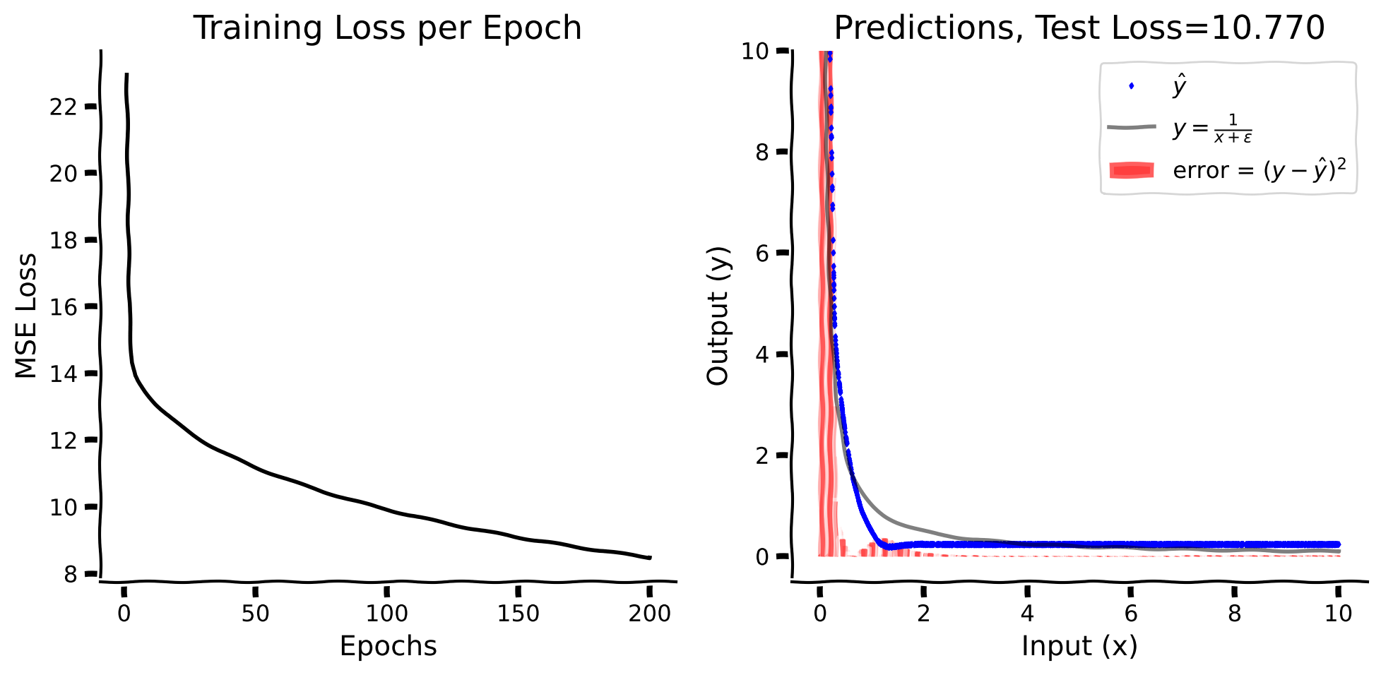
../../../_images/1eb20e890b52eef56066b118eb4b79a9e6611077f388dbda3cdf87616bbba30d.png

While the model learns, we see that it does not fit well with the testing data. Let’s see what are the places where the model struggles during training.

Here, we plot the log mean-squared errors for values of \(x\) between 0 and 1 and their progression with epochs. These are log errors (clipped at \(e^{5}\) represented with blue color).

Plot Training Loss Dynamics#

../../../_images/17232bee8ac4c5da39eb78f689f6774ec2ab99dc30e45743ed7133988876831d.png

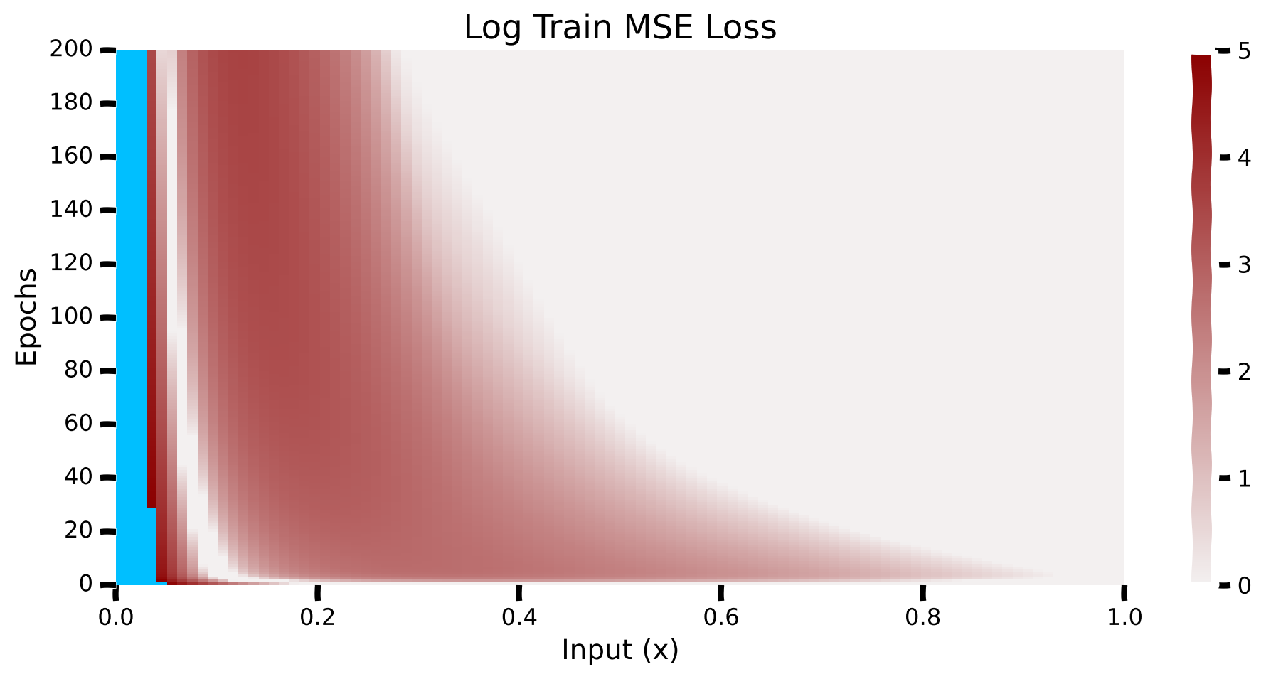
We can see that the model has higher errors for lower values of \(x\), and as the training progresses, the errors for lower \(x\) values start to decrease. Note that the losses are huge for very small values of \(x\) (\(> e^5\)).

Does it mean the model employs more resources to learn the function between 0 and 1?

To check it, let’s visualize the ReLU thresholds.

Vizualize ReLUs#

../../../_images/d0849ec30028d0aa32630e9ba64d53c81a8facc747895529cb8529f2728b45af.png

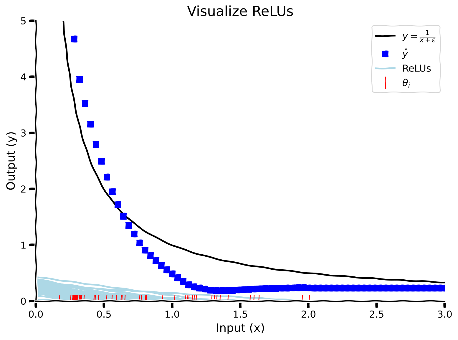
We can see that the thresholds (red lines) are bunched up between 0 and 1, which means that the model dedicates the most resources to learning the function on this interval. Let’s quantify the learning by plotting the threshold distributions and dynamics with epochs.

Here we plot the cumulative distributions of \(\theta_{i}\) & \(w_{i}\). We also plot the values of the parameters as they change across epochs.

Plot Weight Dynamics#

../../../_images/c7d424478d67d31f011ac186f923a95154b161239fec1187a23a5a555087ca5e.png

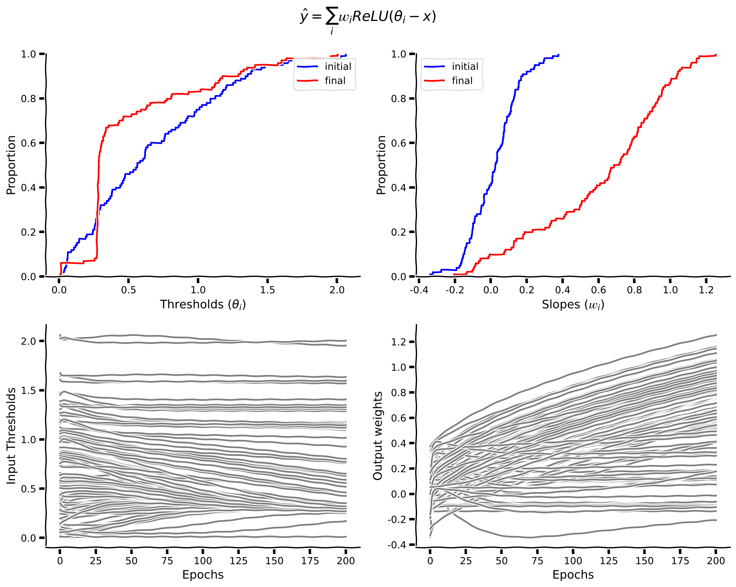
From the cumulative distribution plot of the thresholds (\(\theta_{i}\)), we can see that around \(80%\) of them are below \(x=1\). Hence, the model majorly struggles to learn the function between 0 and 1, where the slope changes a lot.

Since the slope changes infinite times between \(x=0\) and 1, and ReLUs implement a linear function with a single slope, we would ideally need an infinite number of ReLUs units to fit the \(y=\frac{1}{x+\epsilon}\) function. Hence, even though theoretically we can estimate the function, it is not empirically feasible to do so.

Coding Exercise 1 Discussion#

Do you think that having more slope changes in the activation function would help?

Take a minute to think on your own, then discuss in a group.

Submit your feedback#

Coding Exercise 2: Test other non-linear activation functions#

Let’s see if other non-linear activation functions perform better. Specifically, we test:

\(\text{ReLU}(x) = (x)^{+} = \max(0,x)\)
\(\text{ReLU6}(x) = \min(\max(0,x),6)\)
\(\text{SoftPlus}(x, \beta=1) = \frac{1}{\beta} \log(1+e^{βx})\)
\(\text{Sigmoid}(x) = \sigma(x)= \frac{1}{1+e^{-x}}\)
\(\text{Tanh}(x) = \frac{e^{x}-e^{-x}}{e^{x}+e^{-x}}\)

Our model is the same as before, having one layer, except we change the activation function:

\[\hat{y} = \sum_{i}w_{i} \text{Activation}(\theta_{i} - x)\]

Here \(\theta_{i}\) is the threshold, and \(w_{i}\) is the slope of neuron \(i\). We train and evaluate each model three times and plot the mean performance across runs. Your task is to complete the dictionary of the proposed non-linear functions (by defining them using torch.nn library).

###################################################################
## Fill out the following then remove
raise NotImplementedError("Student exercise: complete non-linearities.")
###################################################################
non_linearities = {
    'ReLU': nn.ReLU(),
    'ReLU6': ...,
    'SoftPlus': nn.Softplus(),
    'Sigmoid': ...,
    'Tanh': ...
}

Click for solution

Now, let’s train different networks and evaluate them. Notice that the cell below will run for 1 minute approximately.

Train & Evaluate#

Show code cell source Hide code cell source

# @title Train & Evaluate

class NonLinearNet(nn.Module):
  """
  NonLinearNet architecture
  The structure is the following:
  y = Σi(ai * Non-Linearity(θi - x))
  """
  # Define the structure of your network
  def __init__(self, n_units, non_linearity):
    """
    Args:
      n_units (int): Number of hidden units

    Returns:
      Nothing
    """
    super(NonLinearNet, self).__init__()
    self.n_units = n_units
    self.input_threshold_weights = nn.Parameter(torch.normal(0., 0.1, (self.n_units,)))
    self.non_linearity = non_linearity
    self.output_layer = nn.Linear(n_units, 1)
    nn.init.normal_(self.output_layer.weight, mean=0, std=0.1)

  def forward(self, x):
    """
    Args:
      x: torch.Tensor
        Input tensor of size ([1])
    """
    # Threshold
    op = self.input_threshold_weights - x
    op = self.non_linearity(op)
    op = self.output_layer(op)
    return op

  # Choose the most likely label predicted by the network
  def predict(self, x):
    """
    Args:
      x: torch.Tensor
        Input tensor of size ([1])
    """
    output = self.forward(x)
    return output

# Model
n_units = 1

# Training
n_epochs = 100
learning_rate = 5e-3

# Experiment
n_runs = 3

nls_train_loss_epochs = {}
nls_test_losses = {}

for n_run in range(n_runs):
  for nl_name, nl in non_linearities.items():
    model = NonLinearNet(n_units, nl).to(DEVICE)
    losses_iter, losses_epoch, training_dynamics_mat, \
        input_thresholds_tensor, output_weights_tensor = train_sec1(model, \
        train_dataloader_sec1, learning_rate, n_epochs, VAL_X_LOW, VAL_X_HIGH)
    if nl_name in nls_train_loss_epochs.keys():
      nls_train_loss_epochs[nl_name] = np.vstack((nls_train_loss_epochs[nl_name], np.array(losses_epoch)))
    else:
      nls_train_loss_epochs[nl_name] = np.array(losses_epoch)

    test_loss, x_all, y_all, y_pred_all = evaluate_sec1(model, test_dataloader_sec1)
    if nl_name in nls_test_losses.keys():
      nls_test_losses[nl_name].append(test_loss.item())
    else:
      nls_test_losses[nl_name] = [test_loss.item()]

with plt.xkcd():
    fig, ax = plt.subplots(1, 2, figsize=(10, 5))
    # Plot Training loss
    colors = iter(plt.cm.rainbow(np.linspace(0, 1, len(nls_train_loss_epochs))))
    for nl_ in non_linearities.keys():
      c = next(colors)
      mean_train_loss = np.mean(nls_train_loss_epochs[nl_], axis=0)
      mean_train_loss = np.log(mean_train_loss)
      ax[0].plot(range(1, len(mean_train_loss)+1), mean_train_loss, '-', color=c, label=nl_)
    ax[0].set_xlabel('Epochs')
    ax[0].set_ylabel('Log Mean MSE Loss')
    ax[0].legend()
    ax[0].set_title('Training Loss')

    # Plot loss per epoch
    colors = iter(plt.cm.rainbow(np.linspace(0, 1, len(nls_train_loss_epochs))))
    box = ax[1].boxplot(list(nls_test_losses.values()), showfliers=False, \
                        medianprops={'color':'gray'})
    for median in box['medians']:
      c = next(colors)
      median.set_color(c)
    # plt.ylim((-0.5, 5))
    ax[1].set_xticks(range(1, len(nls_test_losses)+1), labels=nls_test_losses.keys())
    ax[1].set_xlabel('Non Linearity')
    ax[1].set_ylabel('Test MSE Loss')
    ax[1].set_title('Test loss')
    plt.tight_layout()
    plt.show()

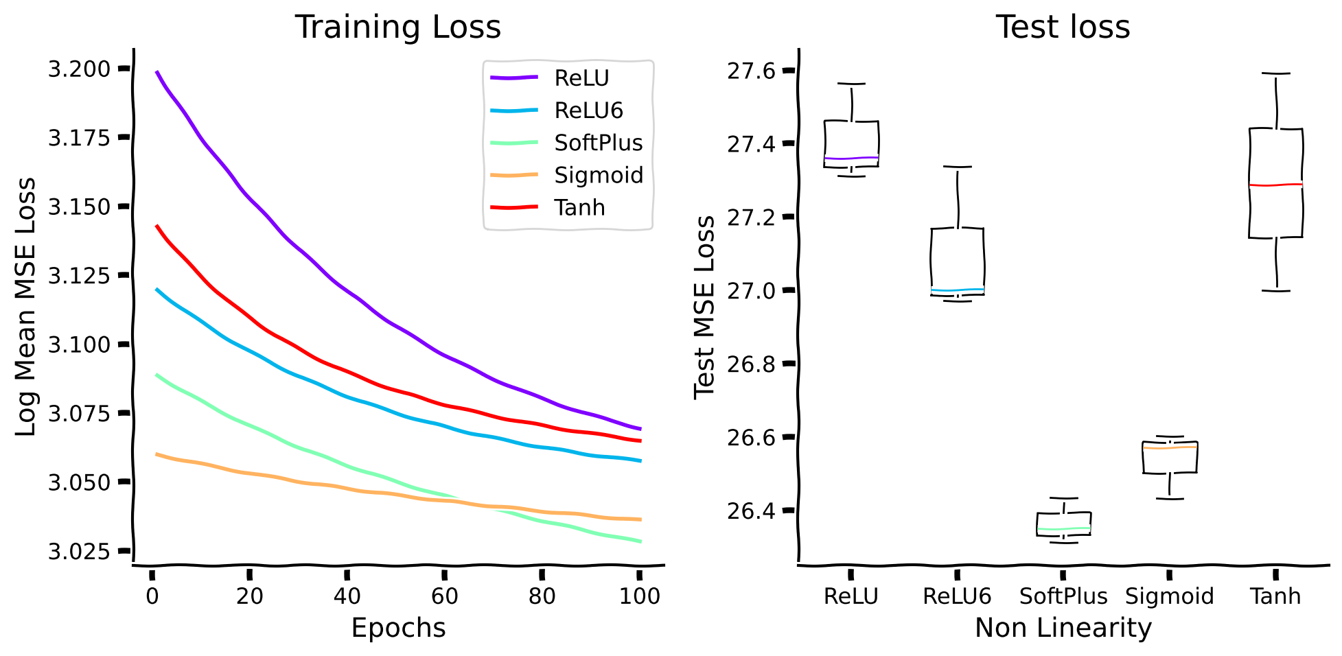
../../../_images/0f59a58068f833db06ce85a01fadeacc03c7ca1286ce2fbfd673700dd1be602c.png

We can see that all of the proposed non-linear activation functions do not perform very well. Hence, it is beneficial to have dedicated computation that implements normalization.

Submit your feedback#

Video 2: Summary#

Submit your feedback#

Section 2: Benefits of normalization#

Estimated timing to here from start of tutorial: 20 minutes.

In this section, we will propose a simple normalization function, which you are going to test in different environments and observe how it is connected to the generalization.

Video 3: Introduction to Normalization#

Submit your feedback#

Subsection 2.1: Explore normalization#

This subsection is devoted to the definition of simple normalization function and the exploration of hyperparameters’ impact on its result.

Coding Exercise 2.1: Implement normalization#

Let’s implement the example of normalization, specifically, we will use the following function:

\[\mathbf{x}_{norm} = \frac{g \mathbf{x}}{\sigma + \sqrt[p]{\Sigma_{i = 1}^{N} |x_{i}|^{p}}}\]

Where

\(x\) is an \(N\)-dimensional vector (\(x \in \mathbb{R}^N\)),
\(g\) is a scaling factor,
\(\sigma\) is a smoothing factor,
\(p\) defines \(p\)-norm of the input vector.

Note that we are normalizing across dimensions (similar to Layer Normalization). You can test your implementation by running the code cell below!

def normalize(x, sigma, p, g):
  """
  Inputs:
  - x(np.ndarray): Input array (n_samples * n_dim)
  - sigma(float): Smoothing factor
  - p(int): p-norm
  - g(int): scaling factor

  Outputs:
  - xnorm (np.ndarray): normalized values.
  """
  #################################################
  ## TODO: Implement the normalization example equation ##
  # Fill remove the following line of code once you have completed the exercise:
  raise NotImplementedError("Student exercise: complete normalization function.")
  #################################################
  # Raise the absolute value of x to the power p
  xp = ...
  # Sum the x over the dimensions (n_dim) axis
  xp_sum = ...
  # Correct the dimensions of xp_sum, and taking the average reduces the dimensions
  # Making xp_sum a row vector of shape (1, n_dim)
  xp_sum = np.expand_dims(xp_sum, axis=1)
  # Raise the sum to the power 1/p and add the smoothing factor (sigma)
  denominator = ...
  # Scale the input data with a factor of g
  numerator = ...
  # Calculate normalized x
  xnorm = numerator/denominator
  return xnorm

Click for solution

Test normalize() function

Submit your feedback#

Interactive Demo 2.1#

Let’s explore the effect of smoothing factor (\(\sigma\)), p-norm (\(p\)) and scaling factor (\(g\)) in our normalization function:

\[\mathbf{x}_{norm} = \frac{g \mathbf{x}}{\sigma + \sqrt[p]{\Sigma_{i = 1}^{N} |x_{i}|^{p}}}\]

We will see the effect of normalization being induced on the points sampled from a 2-dimensional normal distribution.

Take a minute to play around with the values and then discuss them in the group.

Effect of smoothing factor (\(\sigma\)), p-norm (\(p\)) and scaling factor (\(g\))#

Video 4: Effect of smoothing factor, p-norm and scaling factor#

Submit your feedback#

Subsection 2.2: Estimating latent properties#

In this subsection, we will use the normalization function to retrieve the target variable being corrupted with scaling.

Video 5: Normalization example#

Submit your feedback#

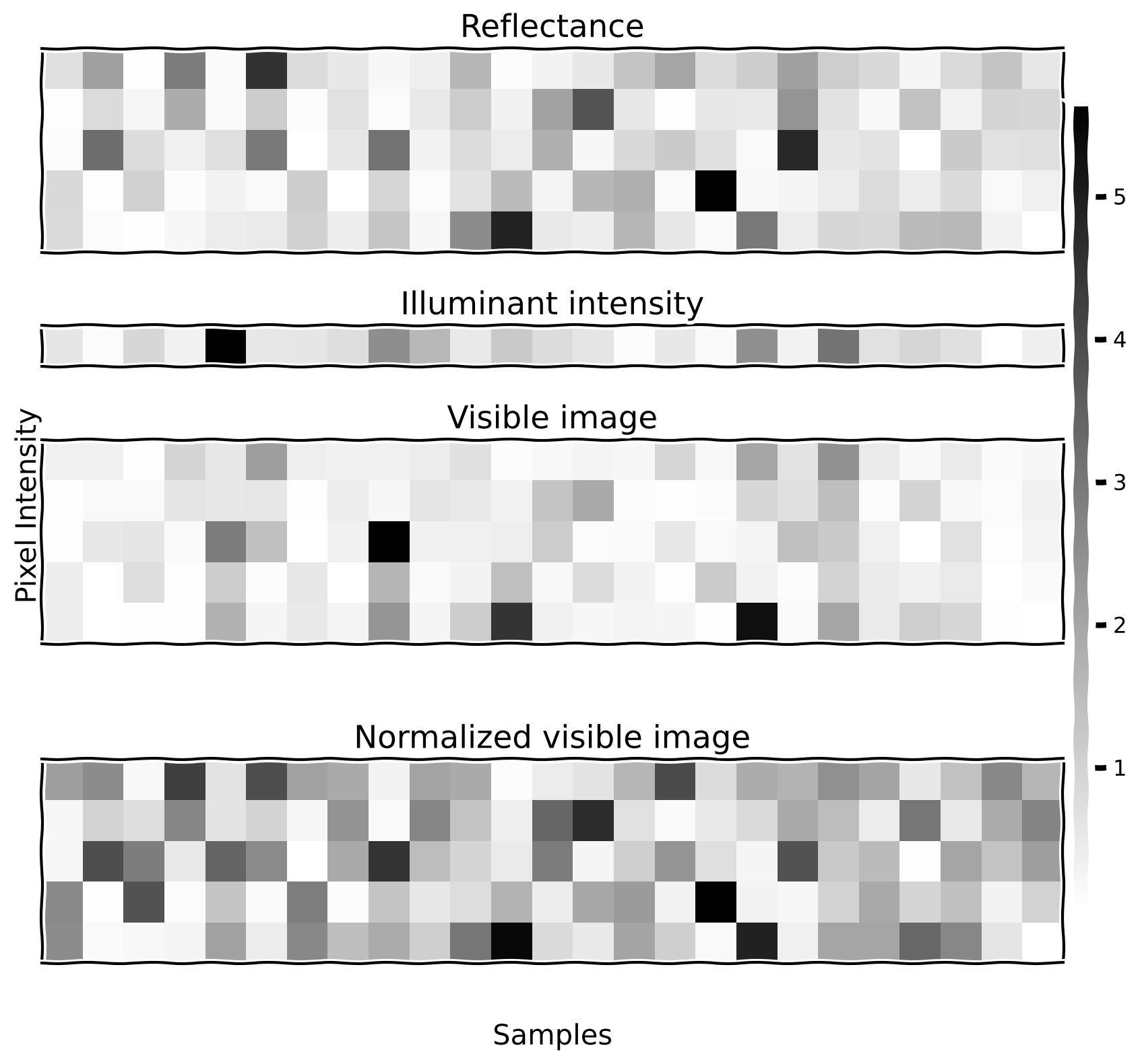
Interactive Demo 2.2.1#

For this demo, we have a target image (\(\mathbf{x}\)), which we would like to infer, and a visible image (\(\mathbf{v}\)), which is a scaled version of the target one: \(\mathbf{x} = s \mathbf{v}\). We will generate 300 different examples (we will visualize only 25 of them) of 5-dimensional vectors \(\mathbf{x}\) (each of the components of the vectors is generated from an exponential distribution with \(\lambda = 1\)). Then, the scaling factor \(s\) is generated from an exponential distribution with \(\lambda = 1\) as well.

Play around with different hyperparameter values to get the best R-squared value.

number_samples = 300 # Number of samples
number_pixels = 5 # Number of pixels per sample

# True reflectance
reflectance = np.random.exponential(1, size=(number_samples, number_pixels))
# Illuminant intensity
illuminant_intensity = np.random.exponential(1, size=(number_samples, 1))
# Visible image
visible_image = np.repeat(illuminant_intensity, number_pixels, axis=1) * reflectance

#################################################
## TODO: Implement the normalization example equation ##
# Fill remove the following line of code one you have completed the exercise:
raise NotImplementedError("Student exercise: choose your parameters values.")
#################################################

# Normalized visible image
norm_visible_image = normalize(
    visible_image,
    sigma = ...,
    p = ...,
    g = ...
)

# Visualize the images
visualize_images_sec22(
    [reflectance, illuminant_intensity, visible_image, norm_visible_image],
    ['Reflectance', 'Illuminant intensity', 'Visible image', 'Normalized visible image'],
    25
)

Click for solution

Example output:

Plot correlation of estimated reflectance with true reflectance#

Submit your feedback#

Interactive Demo 2.2.2#

Now, explore the impact of change in the hyperparemeter values on the R-squared value by using interactive sliders below.

Effect of smoothing factor (\(\sigma\)), p-norm (\(p\)) and scaling factor (\(g\))#

Video 6: Summary#

Submit your feedback#

Subsection 2.3: Layer Normalization#

In this subsection, we are going to explore normalization operation on the real application of a scaled subset of the CIFAR10 dataset.

Video 7: Image recognition example#

Submit your feedback#

First, we fetch the dataset and derive only the part corresponding to three classes: plane, car, and cat.

Get CIFAR3 scaled and unscaled dataloader#

Show code cell source Hide code cell source

# @title Get CIFAR3 scaled and unscaled dataloader

set_seed(seed=42, seed_torch=True)

batch_size = 512

# CIFAR-10 dataset
cifar_transform = transforms.Compose([
    transforms.ToTensor(),
    transforms.Resize((8, 8)),
    transforms.Normalize(
        (0.49139968, 0.48215827, 0.44653124),
        (0.24703233, 0.24348505, 0.26158768))
    ])

cifar10_classes = ('plane', 'car', 'bird', 'cat',
           'deer', 'dog', 'frog', 'horse', 'ship', 'truck')

class CIFAR3(torch.utils.data.Dataset):
    def __init__(self, dataset, classes, scale=False, scaling_limits=[0.05, 0.25]):
        self.dataset = dataset
        self.classes = classes

        # Filter indices based on chosen classes
        cls_indices = {}
        subset_ratio = 0.8
        self.indices = []
        for cls, cls_enum in self.classes.items():
          imgs_ = [i for i, label in enumerate(self.dataset.targets) if label == cls]
          self.indices += imgs_[:int(len(imgs_)*subset_ratio)]

        self.scale = scale
        self.scaling_limits = scaling_limits
        if self.scale:
            self.scale_distribution = torch.distributions.Uniform(*self.scaling_limits)
            self.scale_values = self.scale_distribution.sample((len(self.indices),))

    def __getitem__(self, index_cifar3):
        index_cifar10 = self.indices[index_cifar3]
        image, label = self.dataset[index_cifar10]
        label = self.classes[label]
        if self.scale:
            scalar = self.scale_values[index_cifar3]
            image = image * scalar
        return image, label

    def __len__(self):
        return len(self.indices)

cifar3_classes = {
    0: 0, # plane
    1: 1, # car
    3: 2, # cat
}

# CIFAR-10 datasets
cifar10_trainset = torchvision.datasets.CIFAR10(root='./data', train=True,
                                        download=True, transform=cifar_transform)
cifar10_testset = torchvision.datasets.CIFAR10(root='./data', train=False,
                                       download=True, transform=cifar_transform)

# CIFAR3
cifar3_trainset = CIFAR3(cifar10_trainset, cifar3_classes)
cifar3_trainloader = torch.utils.data.DataLoader(cifar3_trainset, batch_size=batch_size,
                                          shuffle=True)
cifar3_testset = CIFAR3(cifar10_testset, cifar3_classes)
cifar3_testloader = torch.utils.data.DataLoader(cifar3_testset, batch_size=batch_size,
                                         shuffle=False)

# CIFAR3 Scaled
cifar3scaled_trainset = CIFAR3(cifar10_trainset, cifar3_classes, scale=True)
cifar3scaled_trainloader = torch.utils.data.DataLoader(cifar3scaled_trainset, batch_size=batch_size,
                                          shuffle=True)
cifar3scaled_testset = CIFAR3(cifar10_testset, cifar3_classes, scale=True)
cifar3scaled_testloader = torch.utils.data.DataLoader(cifar3scaled_testset, batch_size=batch_size,
                                         shuffle=False)

Downloading https://www.cs.toronto.edu/~kriz/cifar-10-python.tar.gz to ./data/cifar-10-python.tar.gz

Extracting ./data/cifar-10-python.tar.gz to ./data

Files already downloaded and verified

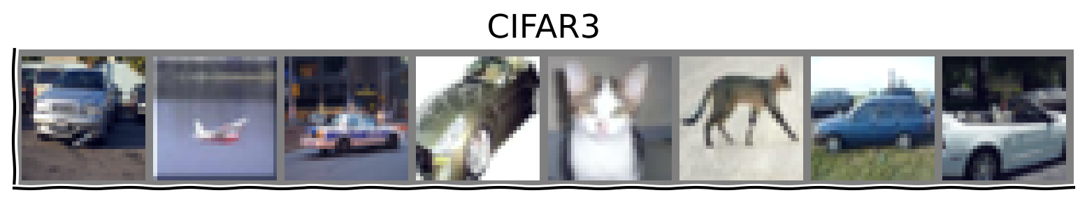
Let us take a look at the original (latent) images and their scaled versions.

Visualize Images#

Show code cell source Hide code cell source

# @title Visualize Images

set_seed(seed=42, seed_torch=True)

num_images_show = 8
cifar_demo_transform = transforms.Compose([
    transforms.ToTensor(),
    transforms.Normalize(
        (0.49139968, 0.48215827, 0.44653124),
        (0.24703233, 0.24348505, 0.26158768))
    ])

# Demo datasets
cifar10_demo_trainset = torchvision.datasets.CIFAR10(root='./data', train=True,
                                        download=True, transform=cifar_demo_transform)
cifar3_demo_trainset = CIFAR3(cifar10_demo_trainset, cifar3_classes)
cifar3scaled_demo_trainset = CIFAR3(cifar10_demo_trainset, cifar3_classes, scale=True)

# functions to show an image
def imshow(img, title):
    with plt.xkcd():
        img = (img * 0.25) + 0.5     # unnormalize
        npimg = img.numpy()
        plt.title(title)
        plt.imshow(np.transpose(npimg, (1, 2, 0)))
        plt.xticks([])
        plt.yticks([])
        plt.show()

# get some random training images
random_idxs = np.random.choice(range(len(cifar3_demo_trainset)), num_images_show)
cifar3_imgs = None
cifar3scaled_imgs = None
cifar3_labels_ = []

for ridx in random_idxs:
    c4img, lbl_ = cifar3_demo_trainset[ridx]
    c4simg, slbl_ = cifar3scaled_demo_trainset[ridx]
    assert lbl_ == slbl_, 'Labels do not match'
    cifar3_labels_.append(lbl_)
    cifar3_imgs = c4img.unsqueeze(0) if (cifar3_imgs is None) else torch.cat((cifar3_imgs, c4img.unsqueeze(0)))
    cifar3scaled_imgs = c4simg.unsqueeze(0) if (cifar3scaled_imgs is None) else torch.cat((cifar3scaled_imgs, c4simg.unsqueeze(0)))

# print labels
print('Labels = ' + ', '.join(f'{cifar10_classes[list(cifar3_classes.keys())[cifar3_labels_[j]]]:5s}' for j in range(num_images_show)))
# show images
imshow(torchvision.utils.make_grid(cifar3_imgs), 'CIFAR3')
# print scaling factor
print('Scaling factors = ' + ', '.join([str(round(i.item(), 3) )for i in cifar3scaled_demo_trainset.scale_values[random_idxs]]))
# show scaled images
imshow(torchvision.utils.make_grid(cifar3scaled_imgs), 'CIFAR3 Scaled')

Files already downloaded and verified

Labels = car  , plane, car  , car  , cat  , cat  , car  , car

../../../_images/b7e6d08b7e9ddc83e410f4497bbd1bab5fdfa9fb3055a8c0494f813cc4ed1cac.png

Scaling factors = 0.14, 0.171, 0.224, 0.148, 0.221, 0.179, 0.099, 0.155

../../../_images/0c493e1b85f9ceccd771d05e83181c4b01ebd9e92efbbc8f916d78c5531e86ff.png

Here, we define the CNN model with an optional parameter for adding the LayerNorm layer.

Define CIFARNet model#

It will take around 3 minutes to complete training on different types of models.

Training & Evaluating the models#

Show code cell source Hide code cell source

# @title Training & Evaluating the models

# Training
n_epochs = 10
learning_rate = 5e-2
momentum = 0.9

# Unscaled CIFAR3
cifar3_net = CIFARNet(layer_norm=False).to(DEVICE)
losses_iter, losses_epoch = train_cnns(cifar3_net, cifar3_trainloader, \
                                  learning_rate, momentum, n_epochs)
# With LayerNorm
cifar3_net_LN = CIFARNet(layer_norm=True).to(DEVICE)
losses_iter_LN, losses_epoch_LN = train_cnns(cifar3_net_LN, cifar3_trainloader, \
                                  learning_rate, momentum, n_epochs)

# Scaled CIFAR3
cifar3scaled_net = CIFARNet(layer_norm=False).to(DEVICE)
losses_iter_scaled, losses_epoch_scaled = train_cnns(cifar3scaled_net, cifar3scaled_trainloader, \
                                  learning_rate, momentum, n_epochs)
# With LayerNorm
cifar3scaled_net_LN = CIFARNet(layer_norm=True).to(DEVICE)
losses_iter_scaled_LN, losses_epoch_scaled_LN = train_cnns(cifar3scaled_net_LN, cifar3scaled_trainloader, \
                                  learning_rate, momentum, n_epochs)

with plt.xkcd():
    # Plot training losses
    fig, ax = plt.subplots(1, 2, figsize=(10, 5))

    # Plot 1 - Unscaled CIFAR3
    # Plot loss per epoch
    ax[0].plot(range(1, len(losses_epoch)+1), np.log(losses_epoch), '-b', label='Without LN')
    ax[0].plot(range(1, len(losses_epoch_LN)+1), np.log(losses_epoch_LN), '-r', label='With LN')
    ax[0].legend()
    ax[0].set_xlabel('Epochs')
    ax[0].set_ylabel('Log Cross Entropy Loss')
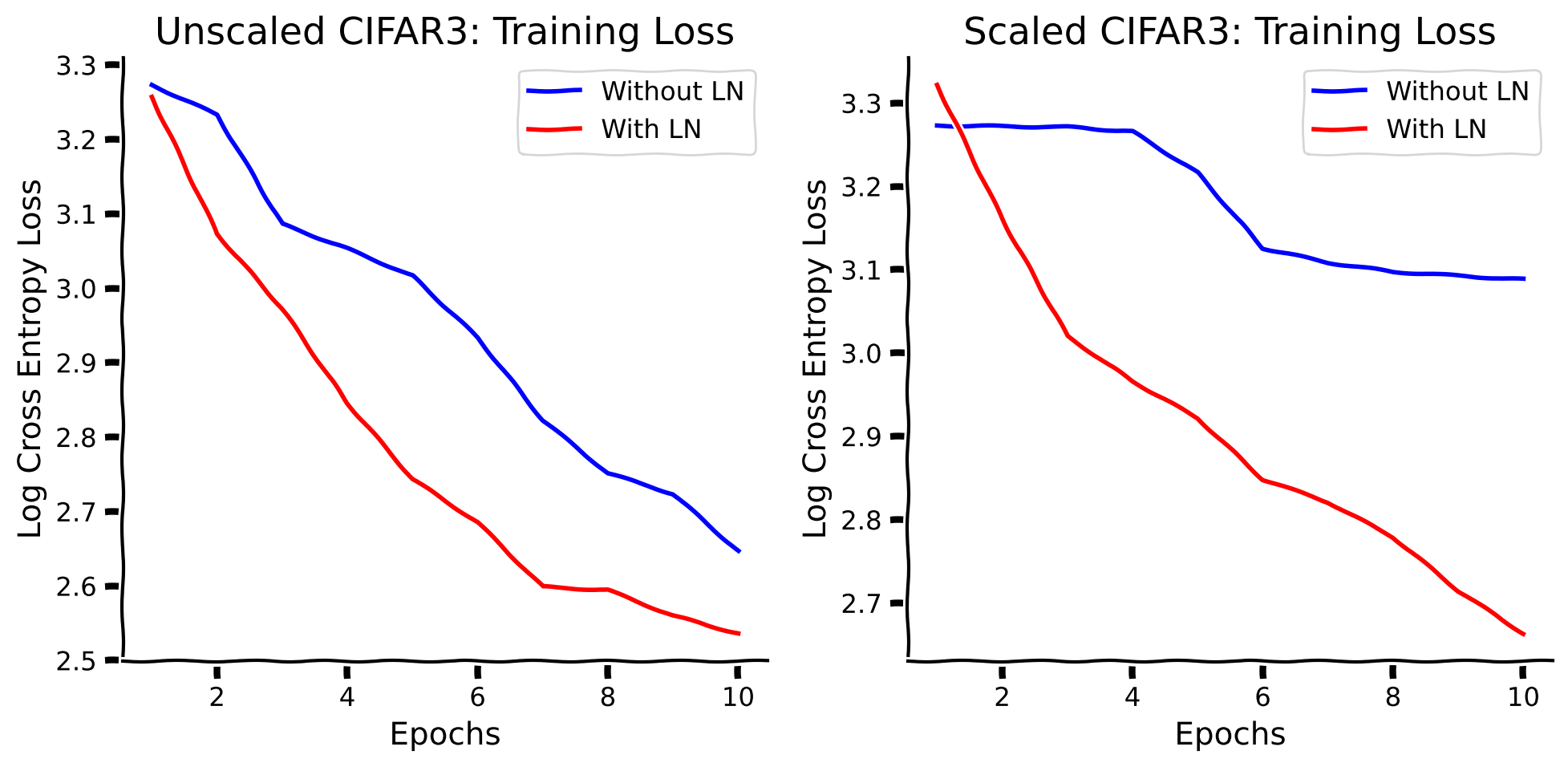
    ax[0].set_title('Unscaled CIFAR3: Training Loss')

    # Plot 2 - Scaled CIFAR3
    # Plot loss per epoch
    ax[1].plot(range(1, len(losses_epoch_scaled)+1), np.log(losses_epoch_scaled), '-b', label='Without LN')
    ax[1].plot(range(1, len(losses_epoch_scaled_LN)+1), np.log(losses_epoch_scaled_LN), '-r', label='With LN')
    ax[1].legend()
    ax[1].set_xlabel('Epochs')
    ax[1].set_ylabel('Log Cross Entropy Loss')
    ax[1].set_title('Scaled CIFAR3: Training Loss')

    plt.tight_layout()
    plt.show()

# Training evaluation
training_loss, training_accuracy = evaluate_cnns(cifar3_net, cifar3_trainloader)
training_loss_LN, training_accuracy_LN = evaluate_cnns(cifar3_net_LN, cifar3_trainloader)
training_loss_scaled, training_accuracy_scaled = evaluate_cnns(cifar3scaled_net, cifar3scaled_trainloader)
training_loss_scaled_LN, training_accuracy_scaled_LN = evaluate_cnns(cifar3scaled_net_LN, cifar3scaled_trainloader)

# Evaluation
test_loss, test_accuracy = evaluate_cnns(cifar3_net, cifar3_testloader)
test_loss_LN, test_accuracy_LN = evaluate_cnns(cifar3_net_LN, cifar3_testloader)
test_loss_scaled, test_accuracy_scaled = evaluate_cnns(cifar3scaled_net, cifar3scaled_testloader)
test_loss_scaled_LN, test_accuracy_scaled_LN = evaluate_cnns(cifar3scaled_net_LN, cifar3scaled_testloader)

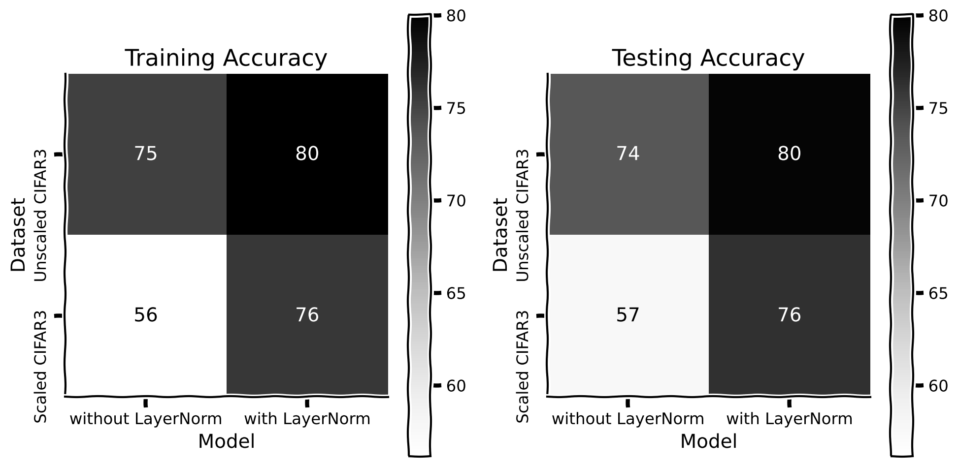
with plt.xkcd():
    # Plot
    fig, axs = plt.subplots(1, 2, figsize=(10, 5))

    training_cm = [[training_accuracy, training_accuracy_LN], [training_accuracy_scaled, training_accuracy_scaled_LN]]
    testing_cm = [[test_accuracy, test_accuracy_LN], [test_accuracy_scaled, test_accuracy_scaled_LN]]
    all_cm = np.array(training_cm+training_cm).flatten()
    vmin = np.min(all_cm)
    vmax = np.max(all_cm)

    training_disp = ConfusionMatrixDisplay(confusion_matrix=np.array(training_cm),
                                   display_labels=['Unscaled CIFAR3', 'Scaled CIFAR3'])
    training_disp.plot(cmap=plt.cm.Greys, ax=axs[0])
    axs[0].images[-1].set_clim(vmin, vmax)
    axs[0].set_yticks([0, 1], ['Unscaled CIFAR3', 'Scaled CIFAR3'], rotation=90)
    axs[0].set_xticks([0, 1], ['without LayerNorm', 'with LayerNorm'])
    axs[0].set_xlabel('Model')
    axs[0].set_ylabel('Dataset')
    axs[0].set_title('Training Accuracy')

    testing_disp = ConfusionMatrixDisplay(confusion_matrix=np.array(testing_cm),
                                   display_labels=['Unscaled CIFAR3', 'Scaled CIFAR3'])
    testing_disp.plot(cmap=plt.cm.Greys, ax=axs[1])
    axs[1].images[-1].set_clim(vmin, vmax)
    axs[1].set_yticks([0, 1], ['Unscaled CIFAR3', 'Scaled CIFAR3'], rotation=90)
    axs[1].set_xticks([0, 1], ['without LayerNorm', 'with LayerNorm'])
    axs[1].set_xlabel('Model')
    axs[1].set_ylabel('Dataset')
    axs[1].set_title('Testing Accuracy')
    plt.tight_layout()
    # Removing shadows from text inside confusion matrix
    for txt in training_disp.text_.flatten():
      txt.set_path_effects([path_effects.Normal()])
    for txt in testing_disp.text_.flatten():
      txt.set_path_effects([path_effects.Normal()])
    plt.show()

../../../_images/283c5c232b2d1b56599dd8291d438501f1b254caeb18e300b61e923786872769.png

../../../_images/60dd0ea73a8d6f490d1f80f1a9c4ac4bdc0cba79a33c5473a96dd88de773093f.png

Let us also check whether normalization improves generalization with different scaling parameters.

Test Generalization#

Show code cell source Hide code cell source

# @title Test Generalization

n_tests = 5

cifar3_scaling_performances = {}
cifar3_scaling_performances_LN = {}

# scaling_limits_tests = [[0.3, 0.5], [0.5, 0.75], [0.75, 1]]
scaling_limits_tests = [[0.4, 0.6], [0.8, 1]]

for test_idx in range(n_tests):
  cifar3_scaled_testloaders = {
    '0.05-0.25 (training range)': cifar3scaled_testloader
  }

  for sc_ in scaling_limits_tests:
    sc_str = '-'.join([str(i) for i in sc_])
    testset_ = CIFAR3(cifar10_testset, cifar3_classes, scale=True, scaling_limits=sc_)
    testloader_ = torch.utils.data.DataLoader(testset_, batch_size=batch_size,
                                          shuffle=False)
    cifar3_scaled_testloaders[sc_str] = testloader_

  for scaling_lims, scaling_testloader in cifar3_scaled_testloaders.items():
    _, noLN_accuracy = evaluate_cnns(cifar3scaled_net, scaling_testloader)
    _, LN_accuracy = evaluate_cnns(cifar3scaled_net_LN, scaling_testloader)
    if scaling_lims in cifar3_scaling_performances.keys():
      cifar3_scaling_performances[scaling_lims] += [noLN_accuracy]
      cifar3_scaling_performances_LN[scaling_lims] += [LN_accuracy]
    else:
      cifar3_scaling_performances[scaling_lims] = [noLN_accuracy]
      cifar3_scaling_performances_LN[scaling_lims] = [LN_accuracy]

with plt.xkcd():
    plt.figure(figsize=(5, 5))
    mean_cifar3_scaling_performances = [np.mean(i) for i in cifar3_scaling_performances.values()]
    std_cifar3_scaling_performances = [np.std(i) for i in cifar3_scaling_performances.values()]
    plt.plot(range(1, len(cifar3_scaled_testloaders)+1), mean_cifar3_scaling_performances, \
             '-.b', label='Without LN')
    plt.errorbar(range(1, len(cifar3_scaled_testloaders)+1), mean_cifar3_scaling_performances, \
             yerr=std_cifar3_scaling_performances, color='b', capsize=5, capthick=2)
    mean_cifar3_scaling_performances_LN = [np.mean(i) for i in cifar3_scaling_performances_LN.values()]
    std_cifar3_scaling_performances_LN = [np.std(i) for i in cifar3_scaling_performances_LN.values()]
    plt.plot(range(1, len(cifar3_scaled_testloaders)+1), mean_cifar3_scaling_performances_LN, \
             '-.r', label='With LN')
    plt.errorbar(range(1, len(cifar3_scaled_testloaders)+1), mean_cifar3_scaling_performances_LN, \
             yerr=std_cifar3_scaling_performances_LN, color='r', capsize=5, capthick=2)
    plt.xticks(range(1, len(cifar3_scaled_testloaders)+1), labels=cifar3_scaled_testloaders.keys())
    plt.xlabel('CIFAR3 scaling range')
    plt.ylabel('Test accuracy')
    plt.title('Testing Generalization for scaled CIFARNet')
    plt.legend()
    plt.show()

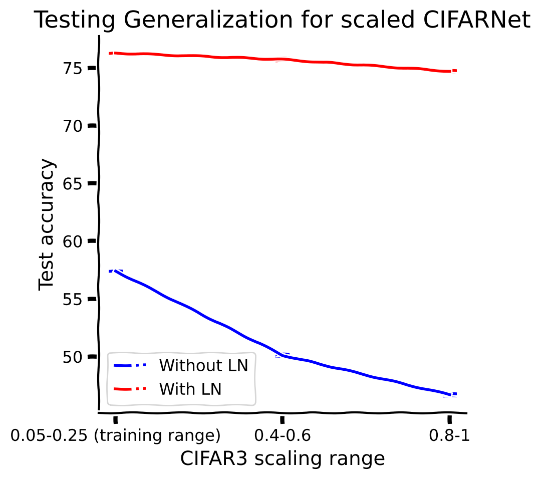
../../../_images/1d59197a0443d82b7efb28191e0a3474efabe7d38105a8cfaaa9823ae497ad64.png

Indeed, by adding a normalization layer, the training process converges quicker, and we achieve better test accuracy as well as better out-of-distribution generalization accuracy in the image recognition tasks.

Submit your feedback#

Video 8: Section summary#

Submit your feedback#

Summary#

Estimated timing of tutorial: 50 minutes

In this tutorial, we observed that normalization as an inductive bias is useful. We have implemented the normalization function and explored the examples. Finally, we discovered the benefits of using normalization.

Video 9: Tutorial summary#

Submit your feedback#

Bonus Section: Benefits of using normalization - Efficient Coding#

Non-linearities are critical for computation, but they can also lose information. We propose you look at a very simple example of how normalization can help preserve information through a network. In the exercise below, complete HardTanh and functions LeakyHardTanh (observe that the inverse of the latter is already here for you).

HardTanh is the function \(f(x)\) which is defined as following:

\[\begin{split}f(x) = \begin{cases} 1, & \text{if } x > 1\\ x, & \text{if } -1 \leq x \leq 1\\ -1, & \text{if } x < -1 \end{cases}\end{split}\]

while LeakyHardTanh is \(f(x) = \text{HardTanh}(x) + \text{leak-slope}* x\).

#################################################
## TODO: Implement the normalization example equation ##
# Fill remove the following line of code once you have completed the exercise:
raise NotImplementedError("Student exercise: complete missing calculations in `HardTanh` and `LeakyHardTanh` functions.")
#################################################

def HardTanh(x):
  """
  Calculate `tanh` output for the given input data.

  Inputs:
  - x (np.ndarray): input data.

  Outputs:
  - output (np.ndarray): `tanh(x)`.
  """
  min_val = -1
  max_val = 1
  output = np.copy(x)
  output[output>...] = ...
  output[output<...] = ...
  return output

def LeakyHardTanh(x, leak_slope=0.03):
  """
  Calculate `tanh` output for the given input data with the leaky term.

  Inputs:
  - x (np.ndarray): input data.
  - leak_slope (float, default = 0.03): leaky term.

  Outputs:
  - output (np.ndarray): `tanh(x)`.
  """
  output = np.copy(x)
  output = HardTanh(output) + ...*...
  return output

def InverseLeakyHardTanh(y, leak_slope=0.03):
  """
  Calculate input into the `tanh` function with the leaky term for the given output.

  Inputs:
  - y (np.array): output of leaky tanh function.
  - leak_slope (float, default = 0.03): leaky term.

  Outputs:
  - output (np.array): input into leaky tanh function.
  """
  ycopy = np.copy(y)
  output = np.where(
      np.abs(ycopy) >= 1+leak_slope, \
      (ycopy - np.sign(ycopy))/leak_slope, \
      ycopy/(1+leak_slope)
  )
  return output

Click for solution

Visualize the functions#

../../../_images/57d3098ed49cef1d5a1d23a61523e8b0d0207c4e10f7fcf58c78e0a0626198de.png

Now, let’s define an \(n\)-dimensional vector \(\mathbf{x}\). This is our target latent variable, and we would like to preserve the information about it. However, \(\mathbf{x}\) is corrupted by a multiplicative scalar nuisance variable, g: \(\mathbf{y}\)=g\(\mathbf{x}\).

Downstream computation will use \(\mathbf{y}\) by passing it through an element-wise non-linearity \(f\) (that saturates beyond a certain input range) and adding noise. By doing so, we lose information – potentially a lot of information if \(g\) is large and pushes the inputs into the saturating part of the non-linearity.

If we knew \(g\), then we could remove it by division and reduce the problem. Although we don’t know \(g\), we can still use Normalization as an estimate of \(g\), divide by that estimate, and invert the non-linearity to recover an approximation of the original \(\mathbf{x}\). Here we use a LeakyHardTanh, which almost saturates but is technically invertible.

Let’s see if Normalization helps. We will compute the correlation between x and the estimate \(\hat{x}\) and compare this correlation with and without the usage of the Normalization function.

Our information (\(\mathbf{X}\)) is a collection of 10-dimensional vectors, having 400 samples in total. \(\mathbf{X} \in \mathbb{R}^{400 \times 10}\), each of the components are drawn from \( \mathcal{N}(0, 1)\). For each component for each vector in \(\mathbf{X}\), we have a nuisance scaling factor \(s \in \mathbb{R}^{400}\), \(s \sim Exp(0.2)\)

Data#

Show code cell source Hide code cell source

# @title Data

def normalize(x, sigma, p, g):
  """
  Inputs:
  - x(np.ndarray): Input array (n_samples * n_dim)
  - sigma(float): Smoothing factor
  - p(int): p-norm
  - g(int): scaling factor

  Outputs:
  - xnorm (np.ndarray): normalized values.
  """
  # Raise the absolute value of x to the power p
  xp = np.power(np.abs(x), p)
  # Sum the x over the dimensions (n_dim) axis
  xp_sum = np.sum(np.power(np.abs(x), p), axis=1)
  # Correct the dimensions of xp_sum, and taking the average reduces the dimensions
  # Making xp_sum a row vector of shape (1, n_dim)
  xp_sum = np.expand_dims(xp_sum, axis=1)
  # Raise the sum to the power 1/p and add the smoothing factor (sigma)
  denominator = sigma + np.power(xp_sum, 1/p)
  # Scale the input data with a factor of g
  numerator = x*g
  # Calculate normalized x
  xnorm = numerator/denominator
  return xnorm

# data
n_samples = 400 # number of samples
n_dim = 10 # dimensions of each sample
latent_std = 1 # width of latent distribution

# nuisance
nuisance_scale = 5 # distribution width for nuisance scaling factor

# normalization
smoothing_factor = 0.1 # normalization smoothness - sigma
norm_p = 2 # Lp norm
norm_scale = 1 # normalization scale

# noise
noise_std = 0.05 # added noise standard deviation

# Non-Linearity
leak_slope = 0.001 # slope after leaky saturation

# random nuisance scaling for each example vector
nuisance = np.random.exponential(nuisance_scale, size=(n_samples, 1))
x_sec31 = np.random.normal(loc=0.0, scale=latent_std, size=(n_samples, n_dim))
y_sec31 = x_sec31 * nuisance # input vectors scaled by random nuisance
ynorm_sec31 = normalize(y_sec31, smoothing_factor, norm_p, norm_scale) * norm_scale # normalized vectors
noise = np.random.normal(loc=0.0, scale=noise_std, size=(n_samples, n_dim))

# without normalization
transmit_noisy_x = LeakyHardTanh(y_sec31, leak_slope) + noise
estimate_x = InverseLeakyHardTanh(transmit_noisy_x, leak_slope)
# with normalization
transmitNormalized_noisy_x = LeakyHardTanh(ynorm_sec31, leak_slope) + noise
estimateNormalized_x = InverseLeakyHardTanh(transmitNormalized_noisy_x, leak_slope)

Let’s take a look at one of the dimensions of \(\mathbf{x}\) and visualize it after nuisance scaling as well as after normalization.

\[\mathbf{x}_{norm} = \frac{g \mathbf{x}}{\sigma + \sqrt[p]{\Sigma_{i = 1}^{N} |x_{i}|^{p}}}\]

Visualize input#

../../../_images/9df52d27fbf4f8189b000bb4dd689ebf8ed874b62cdf9d69b18a9117e13dc462.png

Now, let’s transmit this observable information through a network. In this example, the network is an element-wise LeakyHardTanh. Additionally, the transmission is noisy with transmission noise \(n \sim \mathcal{N}(0, 0.05)\).

Hence, the transmitted signal is LeakyHardTanh(\(s\mathbf{x}\)) + \(n\).

Visualize noisy transmitted signal#

../../../_images/3e4283e6a00c2199d8c09c9d585db1d29a837ff254d16bd7892b6e8e19822c7f.png

Let’s estimate the true information by calculating the inverse of the network (InverseLeakyHardTanh).

Visualize estimated information#

../../../_images/b29ff9fced69ca33ec469348467a03f673bf31e59285b8acd91f3e88cac89be4.png

Let’s quantify how well we can estimate the true information by calculating R-squared values.

Plot correlation between estimated information and true information#

../../../_images/e3af991c4d5d42ee57d502006287b8a80d9fbdc6c4efaaadd37e8eba7989e843.png

We see that normalization helped us preserve the information through transmission by preventing saturation (constraining the information within a limited dynamic range).

Bonus Think 1.1#

We control the dynamic range for normalization. Does there exist an optimum range?

Let’s control the range by manipulating the scaling factor (\(g\)).

\[\mathbf{x}_{norm} = \frac{g \mathbf{x}}{\sigma + \sqrt[p]{\Sigma_{1}^{N} |x_{i}|^{p}}}\]

We will plot the improvement in the correlation versus the range that the normalization produces (via scaling factor \(g\)).

Effect of scaling normalization (\(g\))#

../../../_images/2a51e7e403edaccb6294b7d98af6a97e7eb3a83e7dfe140b5d9782739cb7dc19.png

There’s an optimal normalization range: while being too narrow - the noise dominates, and with too wide - the saturation destroys information.

Bonus Think 1.2#

Thinking deeper: here, we have used normalization only to preserve the information, essentially by avoiding most of the non-linearity. Do you think the computation can gain an advantage by using saturation? How?

Tutorial 2: Normalization

Contents

Tutorial 2: Normalization#

Tutorial Objectives#

Setup#

Install and import feedback gadget#

Imports#

Figure settings#

Helper functions#

Set random seed#

Set device (GPU or CPU)#

Section 1: Can ReLUs implement normalization?#

Video 1: Introduction#

Submit your feedback#

Generate \(y=\frac{1}{x+\epsilon}\) train and test dataloaders#

Coding Exercise 1: ReLUNet#

Training & Evaluating model#

Plot Training Loss Dynamics#

Vizualize ReLUs#

Plot Weight Dynamics#

Coding Exercise 1 Discussion#

Submit your feedback#

Coding Exercise 2: Test other non-linear activation functions#

Train & Evaluate#

Submit your feedback#

Video 2: Summary#

Submit your feedback#

Section 2: Benefits of normalization#

Video 3: Introduction to Normalization#

Submit your feedback#

Subsection 2.1: Explore normalization#

Coding Exercise 2.1: Implement normalization#

Submit your feedback#

Interactive Demo 2.1#

Effect of smoothing factor (\(\sigma\)), p-norm (\(p\)) and scaling factor (\(g\))#

Video 4: Effect of smoothing factor, p-norm and scaling factor#

Submit your feedback#

Subsection 2.2: Estimating latent properties#

Video 5: Normalization example#

Submit your feedback#

Interactive Demo 2.2.1#

Plot correlation of estimated reflectance with true reflectance#

Submit your feedback#

Interactive Demo 2.2.2#

Effect of smoothing factor (\(\sigma\)), p-norm (\(p\)) and scaling factor (\(g\))#

Video 6: Summary#

Submit your feedback#

Subsection 2.3: Layer Normalization#

Video 7: Image recognition example#

Submit your feedback#

Get CIFAR3 scaled and unscaled dataloader#

Visualize Images#

Define CIFARNet model#

Training & Evaluating the models#

Test Generalization#

Submit your feedback#

Video 8: Section summary#

Submit your feedback#

Summary#

Video 9: Tutorial summary#

Submit your feedback#

Bonus Section: Benefits of using normalization - Efficient Coding#

Visualize the functions#

Data#

Visualize input#

Visualize noisy transmitted signal#

Visualize estimated information#

Plot correlation between estimated information and true information#

Bonus Think 1.1#

Effect of scaling normalization (\(g\))#

Bonus Think 1.2#

Submit your feedback#