Tutorial 1: The problem of changing data distributions

Tutorial 1: The problem of changing data distributions#

Week 2, Day 4: Macro-Learning

By Neuromatch Academy

Content creators: Hlib Solodzhuk, Ximeng Mao, Grace Lindsay

Content reviewers: Aakash Agrawal, Alish Dipani, Hossein Rezaei, Yousef Ghanbari, Mostafa Abdollahi, Hlib Solodzhuk, Ximeng Mao, Samuele Bolotta, Grace Lindsay

Production editors: Konstantine Tsafatinos, Ella Batty, Spiros Chavlis, Samuele Bolotta, Hlib Solodzhuk

Tutorial Objectives#

Estimated timing of tutorial: 30 minutes

In this tutorial, we will explore the problems that arise from distribution shifts. Distribution shifts occur when the testing data distribution deviates from the training data distribution; that is, when a model is evaluated on data that somehow differs from what it was trained on.

There are many ways that testing data can differ from training data. Two broad categories of distribution shifts are: covariate shift and concept shift.

In covariate shift, the distribution of input features changes. For example, consider a dog/cat classification task where the model was trained to differentiate between real photos of pets while the testing dataset consists entirely of cartoon characters.

Concept shift, as its name suggests, involves a conceptual change in the relationship between features and the desired output. For example, a recommendation system may learn a user’s preferences, but then those preferences change.

We will explore both types of shifts using a simple function that represents the relationship between the day of the year and the price of fruits in the local market!

Setup#

Install and import feedback gadget#

Imports#

Figure settings#

Plotting functions#

Show code cell source Hide code cell source

# @title Plotting functions

def predict(days, prices, summer_days_mean, summer_days_std, start_month, end_month):
    """
    Predicts the prices for a given date range and plots the true and predicted prices.

    Inputs:
    - days (np.ndarray): input days to predict the prices on.
    - prices (np.ndarray): true price values.
    - summer_days_mean (float): mean value of summer days.
    - summer_days_std (float): standard deviation of summer days.
    - start_month (str): The starting month for the prediction range.
    - end_month (str): The ending month for the prediction range.

    Raises:
    - ValueError: If the specified start_month is after the end_month.
    """

    #check for feasibility of prompt:)
    if months.index(start_month) > months.index(end_month):
        raise ValueError("Please enter valid month interval.")

    #find days and prices for the selected interval
    selected_days = np.expand_dims(days[int(np.sum(months_durations[:months.index(start_month)])) : int(np.sum(months_durations[:months.index(end_month)+1]))], 1)
    selected_prices = prices[int(np.sum(months_durations[:months.index(start_month)])) : int(np.sum(months_durations[:months.index(end_month)+1]))]

    #normalize selected days
    selected_days_norm = (selected_days - summer_days_mean) / summer_days_std

    #evaluate MLP on normalized selected data
    print(f"R-squared value is: {model.score(selected_days_norm, selected_prices):.02f}.")

    #predict for selected dates
    selected_prices_predictions = model.predict(selected_days_norm)

    #plot true and predicted data
    with plt.xkcd():
      plt.plot(selected_days, selected_prices, label = "True Data")
      plt.scatter(selected_days, selected_prices_predictions, label = f"From {start_month} to {end_month} Predictions", marker='o', color='r', zorder=2)
      plt.xlabel('Week')
      plt.ylabel('Price')
      plt.axvspan(days[151], days[242], facecolor='gray', alpha=0.1, label = "Training period")  #add grey background for summer days to see training data
      plt.xlim(np.min(selected_days), np.max(selected_days))
      plt.legend()
      plt.show()

Helper functions#

MLPRegressor(hidden_layer_sizes=(100, 100), max_iter=10000, random_state=42,
             solver='lbfgs')

In a Jupyter environment, please rerun this cell to show the HTML representation or trust the notebook.
On GitHub, the HTML representation is unable to render, please try loading this page with nbviewer.org.

Video 1: Distribution shifts#

Submit your feedback#

Section 1: Covariate shift#

In this section, we are going to discuss the case of covariate shift in distribution - when the distribution of features (usually denoted by $\mathbf{x}$) differs in the training and testing data.

Coding Exercise 1: Fitting pricing data to MLP#

In this exercise, we are going to train a Multi-Layer Perceptron (a fully-connected neural network with non-linear ReLU activation functions) to predict prices for fruits.

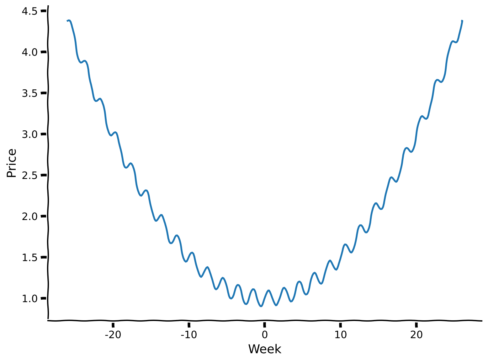
As mentioned in the video, we will model the price of fruits with the following function:

\[f(x) = A x^{2} + B sin(\pi x + \phi) + C\]

This equation suggests quadratic annual behavior (with summer months being at the bottom of the parabola) as well as bi-weekly seasonality introduced by the $sin(\pi x)$ term (with top values being the days where there is supply of fresh fruits to the market). Variables $A, B, \phi \:\: \text{and} \:\: C$ allow us to tune the day-price relation in different scenarios (for example, we will observe the role of $\phi$ in the second section of the tutorial). For this particular case, let us set $A = 0.005$, $B = 0.1$, $\phi = 0$ and $C = 1$.

At first, let’s take a look at the data - we will plot it.

#define variables
A = .005
B = 0.1
phi = 0
C = 1

#define days (observe that those are not 1, ..., 365 but proxy ones to make model function neat)
days = np.arange(-26, 26 + 1/7, 1/7) #defined as fractions of a week

###################################################################
## Fill out the following then remove
raise NotImplementedError("Student exercise: need to complete days-prices relation formula")
###################################################################
prices = ... * ...**2 + ... * np.sin(np.pi * ... + ...) + ...

#plot relation between days and prices
with plt.xkcd():
  plt.plot(days, prices)
  plt.xlabel('Week')
  plt.ylabel('Price')
  plt.show()

Click for solution

Example output:

Let’s ensure that we indeed have 365 days and 26 local maxima (which equals the number of weeks divided by two, as we receive new supplies bi-weekly).

print(f"The number of days is {days.shape[0]}.")

The number of days is 365.

print(f"The number of peaks is {np.sum((np.diff(prices)[:-1] > 0) & (np.diff(prices)[1:] < 0))}.")

The number of peaks is 26.

Notice that x-axis values start from -26 and up to 26, where -26 represents the start of the year season (January), 0 represents the middle of the year (June-July, having the lowest price of the fruits), and 26 ends the year with December. As we have 52 weeks in the year, the value explicitly describes the week before (if it comes with a minus sign) or after the week in the middle of the year.

Now, we are ready to train the model to predict the price of the fruits. First, we will assume we have only been to the market during summer and so only have that data to train on. For this, we need to take data only from the summer months and feed it into the MLP.

As usual, the data will be separated into two distinct classes: train and test. We will measure its performance using the R-squared metric. We will also normalize the data to provide better learning stability for the model.

The MLP consists of two hidden layers, with 100 neurons in each. We use LBFGS as the solver for this particular scenario as it performs better compared to Adam or SGD when the number of data points is limited.

#take only summer data
summer_days = np.expand_dims(days[151:243], 1)
summer_prices = prices[151:243]

#divide data into train and test sets
summer_days_train, summer_days_test, summer_prices_train, summer_prices_test = train_test_split(summer_days, summer_prices, random_state = 42)

###################################################################
## Fill out the following then remove
raise NotImplementedError("Student exercise: need to normalized days and to fit model with it")
###################################################################

#apply normalization for days
summer_days_mean, summer_days_std = np.mean(...), np.std(...)
summer_days_train_norm = (summer_days_train - ...) / ...
summer_days_test_norm = (summer_days_test - ...) / ...

#define MLP
model = MLPRegressor(hidden_layer_sizes=(100, 100), max_iter=10000, random_state = 42, solver = "lbfgs") # LBFGS is better to use when there is small amount of data

#train MLP
model.fit(..., ...)

#evaluate MLP on test data
print(f"R-squared value is: {model.score(summer_days_test_norm, summer_prices_test):.02f}.")

Click for solution

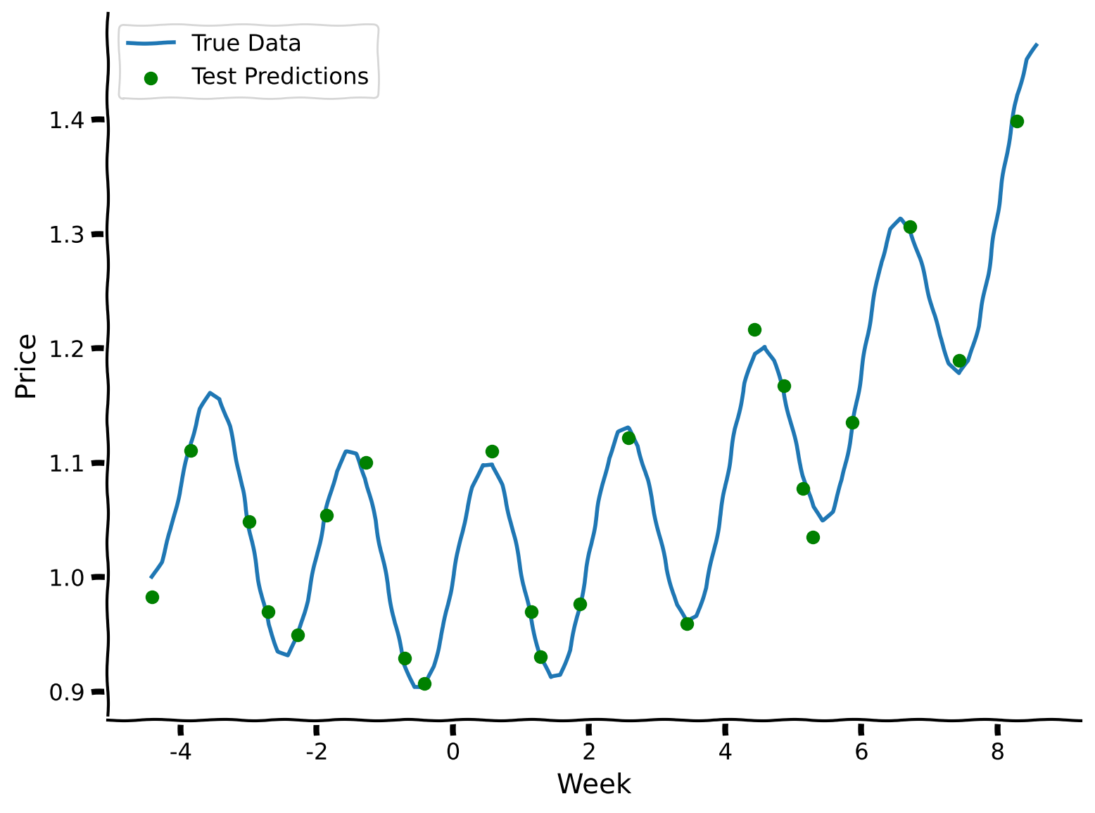
Let’s explore the predictions of the model visually.

Make sure you execute this cell to observe the plot!#

../../../_images/13fc9dea26c2eaf6466673da47e7a2925ead093e9865f67cfd4ded2bc27cc670.png

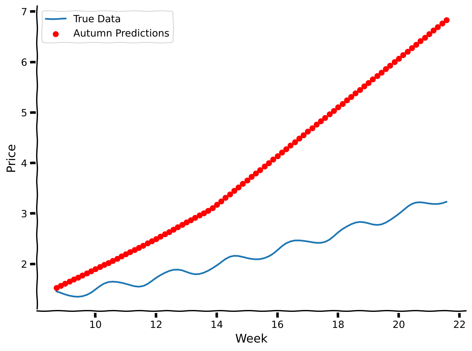
Now that we’ve learned about prices during the summer, can we predict what prices will be in autumn? Let’s see how well our summer-trained model performs.

#take only autumn data
autumn_days = np.expand_dims(days[243:334], 1)
autumn_prices = prices[243:334]

#apply normalization (pay attention to the fact that we use summer metrics as the model was trained on them!)
autumn_days_norm = (autumn_days - summer_days_mean) / summer_days_std

#evaluate MLP on normalized autumn data
print(f"R-squared value is: {model.score(autumn_days_norm, autumn_prices):.02f}.")

R-squared value is: -10.79.

The R-squared value dropped significantly; let’s observe what is going on visually.

Make sure you execute this cell to observe the plot!#

../../../_images/f78ec67f05c752fe27d07ba9877d9d318c9d8003e5042577d3e991b6adcb28e3.png

Coding Exercise 1 Discussion#

How would you qualitatively evaluate the model’s performance on autumn data? Does it capture the annual trend? Does it capture the weekly trend?

Click for solution

Submit your feedback#

Interactive Demo 1: Covariate shift impact on predictability power#

In this interactive demo, you will explore how well the model generalizes to other months using two dropdown menus for selecting the start and end months for testing data.

!N.B.: Note that for summer months, some training data will also be included in the evaluation of the prediction.

Make sure you execute this cell to enable the widget!

Interactive Demo 1 Discussion#

Does the amount of covariate shift impact the model’s performance? What happens at the borders of the training period—does the model still capture the dynamics right before and after it?

Click for solution

Submit your feedback#

Section 2: Concept shift#

Estimated time to reach this point from the start of the tutorial: 15 minutes

In this section, we are going to explore another case of distribution shift, which is different in nature from covariate shift: concept shift.

Exercise 2: Change in the day of supply#

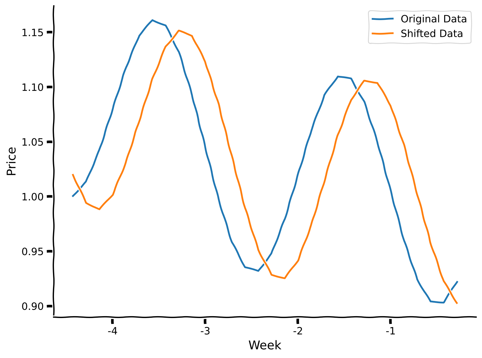
We observed how transitioning from summer to autumn introduces covariate shifts, but what would lead to a concept shift in our fruit price relationship? One possibility is a change in the day of the week when fresh fruits are delivered. Let’s revisit the modeling equation:

\[f(x) = A x^{2} + B sin(\pi x + \phi) + C\]

Which variable, do you think, needs to be changed so that we now receive fresh fruits 2 days later than before?

Answer

Yes, indeed, it involves a sinusoidal phase shift — we only need to change the $\phi$ value.

Let’s take a look at how well the model generalizes to this unexpected change as well.

shifted_phi = - 2 * np.pi / 7
shifted_prices = A * days**2 + B * np.sin(np.pi*days + shifted_phi) + C

#plot relation between days, prices & shifted prices for June
with plt.xkcd():
  plt.plot(days[151:181], prices[151:181], label = "Original Data")
  plt.plot(days[151:181], shifted_prices[151:181], label = "Shifted Data")
  plt.xlabel('Week')
  plt.ylabel('Price')
  plt.legend()
  plt.show()

../../../_images/69dece28d0de8f4aa8a99c5637622707a31fb48bbf33bdc5f648f7aebf804491.png

#take only summer shifted data
summer_days = np.expand_dims(days[151:243], 1)
summer_prices_shifted = shifted_prices[151:243]

#apply normalization (pay attention to the fact that we use summer metrics as the model was trained on them!)
summer_days_norm = (summer_days - summer_days_mean) / summer_days_std

#evaluate MLP on normalized original & shifted data
print(f"R-squared value for original prices is: {model.score(summer_days_norm, summer_prices):.02f}.")
print(f"R-squared value for shifted prices is: {model.score(summer_days_norm, summer_prices_shifted):.02f}.")

R-squared value for original prices is: 1.00.
R-squared value for shifted prices is: 0.75.

Make sure you execute this cell to observe the plot!#

../../../_images/099e82af4251506caeecd517206d3e2370e484d5fc305348ddddc23e04fc9d13.png

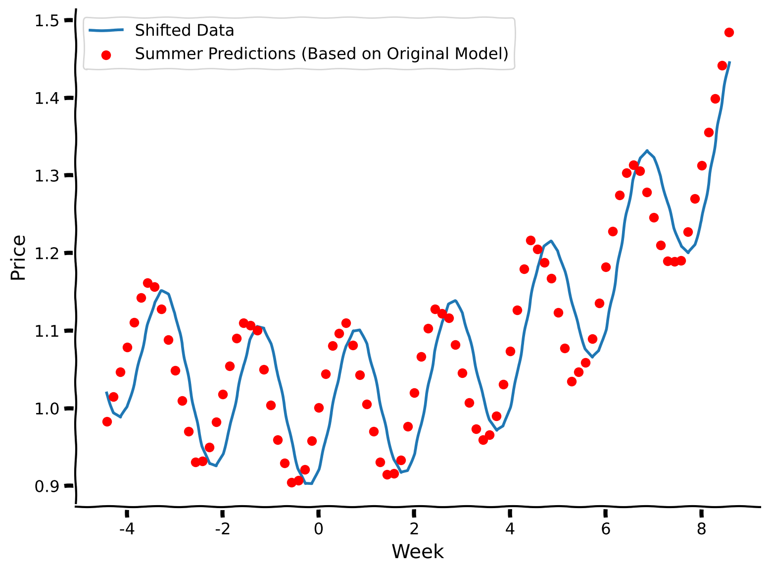
Indeed, the model’s predictions are capturing the original phase, not the phase-shifted function. Well, it’s somewhat expected: we fixed values of features (in this case, week number), trained at first on one set of output values (prices), and then changed the outputs to measure the model’s performance. It’s obvious that the model will perform badly. Still, it’s important to notice the effect of concept shift and this translation between conceptual effect and its impact on modeling.

Exercise 2 Discussion#

Why do you think the R-squared value is still higher for this particular example of concept shift compared to the covariate shift?

Click for solution

Submit your feedback#

Think!: Examples of concept shift#

What other examples of concept shift could you come up with in the context of the “fruit prices” task? What variables would these shifts impact?

Take 2 minutes to think, then discuss as a group.

Submit your feedback#

Summary#

Estimated timing of tutorial: 30 minutes

Here’s what we learned:

Covariate and concept shifts are two different types of data distribution shifts.
Distribution shifts negatively impact model performance.

In the next tutorials, we are going to address the question of generalization—what are the techniques and methods to deal with poor generalization performance due to distribution shifts.

Tutorial 1: The problem of changing data distributions

Contents

Tutorial 1: The problem of changing data distributions#

Tutorial Objectives#

Setup#

Install and import feedback gadget#

Imports#

Figure settings#

Plotting functions#

Helper functions#

Video 1: Distribution shifts#

Submit your feedback#

Section 1: Covariate shift#

Coding Exercise 1: Fitting pricing data to MLP#

Make sure you execute this cell to observe the plot!#

Make sure you execute this cell to observe the plot!#

Coding Exercise 1 Discussion#

Submit your feedback#

Interactive Demo 1: Covariate shift impact on predictability power#

Interactive Demo 1 Discussion#

Submit your feedback#

Section 2: Concept shift#

Exercise 2: Change in the day of supply#

Make sure you execute this cell to observe the plot!#

Exercise 2 Discussion#

Submit your feedback#

Think!: Examples of concept shift#

Submit your feedback#

Summary#