Tutorial 3: Neural network modularity#
Week 2, Day 1: Macrocircuits
By Neuromatch Academy
Content creators: Ruiyi Zhang
Content reviewers: Xaq Pitkow, Hlib Solodzhuk, Patrick Mineault, Alex Murphy
Production editors: Konstantine Tsafatinos, Ella Batty, Spiros Chavlis, Samuele Bolotta, Hlib Solodzhuk, Alex Murphy
Tutorial objectives#
Estimated timing of tutorial: 1 hour
This tutorial will exemplify the importance of modularity in neural network architecture. We will train deep reinforcement learning (RL) agents with two types of neural network architectures, one modular and the other holistic, in a neuroscience navigation task.
As you have learned in previous lectures, better learning and generalization are important benefits of an appropriate inductive bias. This applies to both biological and artificial learning systems. Indeed, it has been shown that macaques trained in this navigation task can master the training task well and generalize to novel tasks derived from it. Since the brain is quite modular, it will be interesting to see if artificial models with a more modular architecture also allow for better learning and generalization than those with a less modular, holistic architecture.
Our learning objectives for today are:
Build RL agents with different neural architectures for a spatial navigation task.
Compare the differences in learning between RL agents with different architectures.
Compare the differences in generalization between RL agents with different architectures.
Use neural decoding to understand why the modular architecture for this specific task is advantageous.
Keep the No-Free-Lunch Theorem in mind: the benefits of a modular architecture for one task cannot apply to all possible tasks.
This tutorial is based on this paper.
Setup#
Install and import feedback gadget#
Show code cell source
# @title Install and import feedback gadget

!pip install vibecheck datatops --quiet
!pip install pandas --quiet
!pip install scikit-learn --quiet

from vibecheck import DatatopsContentReviewContainer
def content_review(notebook_section: str):
    return DatatopsContentReviewContainer(
        "",  # No text prompt
        notebook_section,
        {
            "url": "https://pmyvdlilci.execute-api.us-east-1.amazonaws.com/klab",
            "name": "neuromatch_neuroai",
            "user_key": "wb2cxze8",
        },
    ).render()

feedback_prefix = "W2D1_T3"
Imports#
Show code cell source
# @title Imports

#plotting
import matplotlib.pyplot as plt
from matplotlib.ticker import FuncFormatter
from matplotlib.patches import Circle

#modeling
from scipy.stats import sem
from sklearn.linear_model import LinearRegression, Ridge
import torch
import torch.nn as nn
import torch.nn.functional as F
import numpy as np
import pandas as pd

#utils
from tqdm.notebook import tqdm
import pickle
import logging
import os
from pathlib import Path
import requests
import hashlib
import zipfile
Figure settings#
Show code cell source
# @title Figure settings

logging.getLogger('matplotlib.font_manager').disabled = True

%matplotlib inline
%config InlineBackend.figure_format = 'retina' # perfrom high definition rendering for images and plots
plt.style.use("https://raw.githubusercontent.com/NeuromatchAcademy/course-content/main/nma.mplstyle")
Helper functions#
Show code cell source
# @title Helper functions

def my_tickformatter(value, pos):
    if abs(value) > 0 and abs(value) < 1:
        value = str(value).replace('0.', '.').replace('-', '\u2212')
    elif value == 0:
        value = 0
    elif int(value) == value:
        value = int(value)
    return value

def cart2pol(x, y):
    rho = np.sqrt(x**2 + y**2)
    phi = np.arctan2(y, x)
    return rho, phi

def get_neural_response(agent, df):
    responses = []
    with torch.no_grad():
        for _, trial in df.iterrows():
            response = agent.actor.rnn(trial.state_input)[0]
            responses.append(response.squeeze(1))
        df['response'] = responses

def fit_decoder(trajectory, variables=['pos_x', 'pos_y'], train_frac=0.7):
    key = 'response'
    train_trajectory = trajectory[:round(len(trajectory) * train_frac)]
    train_X = np.vstack(train_trajectory[key])
    test_trajectory = trajectory[round(len(trajectory) * train_frac):]
    test_X = np.vstack(test_trajectory[key])

    y = train_trajectory[variables].values
    train_y = np.vstack([np.hstack([v for v in y[:, i]]) for i in range(y.shape[1])]).T
    y = test_trajectory[variables].values
    test_y = np.vstack([np.hstack([v for v in y[:, i]]) for i in range(y.shape[1])]).T

    decoder = Ridge(alpha=0.1)
    decoder.fit(train_X, train_y)

    return decoder, test_X, test_y

def filter_fliers(data, whis=1.5, return_idx=False):
    if not isinstance(data, list):
        data = [data]
    filtered_data = []; data_ides = []
    for value in data:
        Q1, Q2, Q3 = np.percentile(value, [25, 50, 75])
        lb = Q1 - whis * (Q3 - Q1); ub = Q3 + whis * (Q3 - Q1)
        filtered_data.append(value[(value > lb) & (value < ub)])
        data_ides.append(np.where((value > lb) & (value < ub))[0])
    if return_idx:
        return filtered_data, data_ides
    else:
        return filtered_data
Plotting functions#
Show code cell source
# @title Plotting functions

major_formatter = FuncFormatter(my_tickformatter)
modular_c = 'lightseagreen'; holistic_c = 'salmon'
reward_c = 'rosybrown'; unreward_c = 'dodgerblue'

fontsize = 7
lw = 1

def set_violin_plot(vp, facecolor, edgecolor, linewidth=1, alpha=1, ls='-', hatch=r''):
    with plt.xkcd():
        plt.setp(vp['bodies'], facecolor=facecolor, edgecolor=edgecolor,
                 linewidth=linewidth, alpha=alpha ,ls=ls, hatch=hatch)
        plt.setp(vp['cmins'], facecolor=facecolor, edgecolor=edgecolor,
                 linewidth=linewidth, alpha=alpha)
        plt.setp(vp['cmaxes'], facecolor=facecolor, edgecolor=edgecolor,
                 linewidth=linewidth, alpha=alpha)
        plt.setp(vp['cbars'], facecolor='None', edgecolor='None',
                 linewidth=linewidth, alpha=alpha)

        linecolor = 'k' if facecolor == 'None' else 'snow'
        if 'cmedians' in vp:
            plt.setp(vp['cmedians'], facecolor=linecolor, edgecolor=linecolor,
                     linewidth=linewidth, alpha=alpha, ls=ls)
        if 'cmeans' in vp:
            plt.setp(vp['cmeans'], facecolor=linecolor, edgecolor=linecolor,
                     linewidth=linewidth, alpha=alpha, ls=ls)
Set random seed#
Show code cell source
# @title Set random seed

import random
import numpy as np

def set_seed(seed=None, seed_torch=True):
  if seed is None:
    seed = np.random.choice(2 ** 32)
  random.seed(seed)
  np.random.seed(seed)
  if seed_torch:
    torch.manual_seed(seed)
    torch.cuda.manual_seed_all(seed)
    torch.cuda.manual_seed(seed)
    torch.backends.cudnn.benchmark = False
    torch.backends.cudnn.deterministic = True

set_seed(seed = 42)
Data retrieval#
Show code cell source
# @title Data retrieval

def download_file(fname, url, expected_md5):
    """
    Downloads a file from the given URL and saves it locally.
    """
    if not os.path.isfile(fname):
        try:
            r = requests.get(url)
        except requests.ConnectionError:
            print("!!! Failed to download data !!!")
            return
        if r.status_code != requests.codes.ok:
            print("!!! Failed to download data !!!")
            return
        if hashlib.md5(r.content).hexdigest() != expected_md5:
            print("!!! Data download appears corrupted !!!")
            return
        with open(fname, "wb") as fid:
            fid.write(r.content)

def extract_zip(zip_fname):
    """
    Extracts a ZIP file to the current directory.
    """
    with zipfile.ZipFile(zip_fname, 'r') as zip_ref:
        zip_ref.extractall(".")

# Details for the zip files to be downloaded and extracted
zip_files = [
    {
        "fname": "agents.zip",
        "url": "https://osf.io/v9xqp/download",
        "expected_md5": "2cd35da7ea34e10e6ed2e7c983f0b908"
    },
    {
        "fname": "training_curve.zip",
        "url": "https://osf.io/9kjy4/download",
        "expected_md5": "eb7e07398aa12bd0fd9cf507d9a142c6"
    }
]

# New addition for other files to be downloaded, specifically non-zip files
model_files = [
    {
        "fname": "holistic_dfs.pkl",
        "url": "https://osf.io/9h7tq/download",
        "expected_md5": "92d0adb175724641590a611c48d721cc"
    },
    {
        "fname": "holistic_dfs_2x.pkl",
        "url": "https://osf.io/ybdmp/download",
        "expected_md5": "173e13bea9c2bbe8737a40e0d36063d4"
    },
    {
        "fname": "modular_dfs.pkl",
        "url": "https://osf.io/apkym/download",
        "expected_md5": "38a4603464b3e4351bd56625d24d5e16"
    },
    {
        "fname": "modular_dfs_2x.pkl",
        "url": "https://osf.io/wqbe2/download",
        "expected_md5": "5f19bafa3308f25ca163c627b7d9f63f"
    }
]

# Process zip files: download and extract
for zip_file in zip_files:
    download_file(zip_file["fname"], zip_file["url"], zip_file["expected_md5"])
    extract_zip(zip_file["fname"])

# Process model files: download only
for model_file in model_files:
    download_file(model_file["fname"], model_file["url"], model_file["expected_md5"])
Video 1: Introduction#
Submit your feedback#
Show code cell source
# @title Submit your feedback
content_review(f"{feedback_prefix}_introduction")
Section 2: Evaluate agents in the training task#
Estimated timing to here from start of tutorial: 25 minutes
With the code for the environment and agents complete, we will now write an evaluation function allowing the agent to interact with the environment where the quality of the model can be assessed.
Coding Exercise 3: Evaluation function#
We first sample 1,000 targets for the RL agent to steer towards.
Sample 1000 targets#
Show code cell source
# @title Sample 1000 targets
arg = Config()

set_seed(0)
env = Env(arg)
target_positions = []

for _ in range(1000):
    __ = env.reset()
    target_positions.append(env.target_position)
Then, we define the evaluation function. For each target, an agent takes multiple steps to steer to it. In each step, the agent selects an action based on the input information about the state, and the environment updates according to the agent’s action.
Fill in the missing code that calculates the reward.
def evaluation(agent, gain_factor=1):
    """
    Evaluates the agent's performance in the environment.

    Inputs:
    - agent (Agent): The agent to be evaluated.
    - gain_factor (float): A factor to scale the process gain. Default is 1.

    Outputs:
    - results (DataFrame): A DataFrame containing evaluation results with columns:
      - 'pos_x': List of x positions over episodes.
      - 'pos_y': List of y positions over episodes.
      - 'pos_r_end': List of final radial distances from origin over episodes.
      - 'target_x': List of target x positions.
      - 'target_y': List of target y positions.
      - 'target_r': List of target radial distances.
      - 'rewarded': List of binary rewards indicating if the target was reached and stopped.
      - 'state_input': List of state inputs recorded during the episodes.
    """
    set_seed(0)
    env = Env(arg)

    pos_x = []; pos_y = []; pos_r_end = []
    target_x = []; target_y = []; target_r = []
    rewarded = []; state_input_ = []

    for target_position in tqdm(target_positions):
        state = env.reset(target_position=target_position, gain=arg.process_gain_default * gain_factor)
        agent.obs_step.reset(env.gain)

        state_input = torch.cat([torch.zeros([1, 1, arg.OBS_DIM]), torch.zeros([1, 1, arg.ACTION_DIM]),
                                 env.target_position_obs.view(1, 1, -1)], dim=2)
        hidden_in = (torch.zeros(1, 1, agent.actor.RNN_SIZE), torch.zeros(1, 1, agent.actor.RNN_SIZE))

        state_inputs = []
        states = []

        for t in range(arg.EPISODE_LEN):
            # 1. Agent takes an action given the state-related input
            action, hidden_out = agent.select_action(state_input, hidden_in)

            # 2. Environment updates to the next state given state and action,
            #    as well as checking if the agent has reached the reward zone,
            #    and if the agent has stopped.
            next_state, reached_target = env(state, action, t)
            is_stop = env.is_stop(action)

            # 3. Receive reward
            ###################################################################
            ## Fill out the following then remove
            raise NotImplementedError("Student exercise: compute the reward.")
            ###################################################################
            # TODO: Compute the reward. The reward is '1' when the target is reached and the agent stops on it,
            # otherwise, the reward is '0'.
            # Hint: Use variables 'reached_target' and 'is_stop'.
            reward = ...

            # 4. Agent observes the next state and constructs the next state-related input
            next_observation = agent.obs_step(next_state)
            next_state_input = torch.cat([next_observation.view(1, 1, -1), action,
                                          env.target_position_obs.view(1, 1, -1)], dim=2)

            states.append(state)
            state_inputs.append(state_input)

            state_input = next_state_input
            state = next_state
            hidden_in = hidden_out

            # trial is done when the agent stops
            if is_stop:
                break

        # store data for each trial
        pos_x_, pos_y_, _, _, _ = torch.chunk(torch.cat(states, dim=1), state.shape[0], dim=0)
        pos_x.append(pos_x_.view(-1).numpy() * arg.LINEAR_SCALE)
        pos_y.append(pos_y_.view(-1).numpy() * arg.LINEAR_SCALE)

        pos_r, _ = cart2pol(pos_x[-1], pos_y[-1])
        pos_r_end.append(pos_r[-1])

        target_x.append(target_position[0].item() * arg.LINEAR_SCALE)
        target_y.append(target_position[1].item() * arg.LINEAR_SCALE)
        target_r_, _ = cart2pol(target_x[-1], target_y[-1])
        target_r.append(target_r_)

        state_input_.append(torch.cat(state_inputs))
        rewarded.append(reward.item())

    return(pd.DataFrame().assign(pos_x=pos_x, pos_y=pos_y,
                                 pos_r_end=pos_r_end, target_x=target_x, target_y=target_y,
                                 target_r=target_r, rewarded=rewarded,
                                 state_input=state_input_))
Since training RL agents takes a lot of time, here we load the pre-trained modular and holistic agents and evaluate these two agents on the same sampled 1,000 targets. We will then store the evaluation data in pandas Dataframe object.
modular_agent = Agent(arg, ModularActor)
modular_agent.load(Path('agents/modular'), 0)
modular_df = evaluation(modular_agent)
holistic_agent = Agent(arg, HolisticActor)
holistic_agent.load(Path('agents/holistic'), 0)
holistic_df = evaluation(holistic_agent)
Submit your feedback#
Show code cell source
# @title Submit your feedback
content_review(f"{feedback_prefix}_evaluation_function")
Coding Exercise 4: Agent trajectory in a single trial#
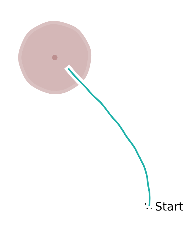
After evaluation, we want to visualize the agents’ steering trajectories. Fill in the missing code to compute the distance between the stop location and the target location. Given the reward boundary is \(65\) cm, are these trials rewarded?
Modular agent trajectory#
with plt.xkcd():
    trial_idx = 21
    trial = modular_df.iloc[trial_idx]

    fig = plt.figure(figsize=(2.2, 1.7), dpi=200)
    ax = fig.add_subplot(111)

    ax.set_aspect('equal')
    ax.spines['top'].set_visible(False)
    ax.spines['right'].set_visible(False)
    ax.spines['bottom'].set_visible(False)
    ax.spines['left'].set_visible(False)
    ax.axes.xaxis.set_ticks([]); ax.axes.yaxis.set_ticks([])

    # plot trajectory
    px = trial.pos_x; py = trial.pos_y
    ax.plot(px, py, lw=lw, c=modular_c)

    # plot target
    target_x = trial.target_x; target_y = trial.target_y
    print(f'Target distance from the start location: {np.around(trial.target_r, 1)} cm')

    ###################################################################
    ## Fill out the following then remove
    raise NotImplementedError("Student exercise: calculate the distance between target location and stop position.")
    ###################################################################
    # Given target locations as trial.target_x and trial.target_y,
    # and stop locations as trial.pos_x[-1] and trial.pos_y[-1],
    # compute the Euclidean distance between the target and stop locations.
    distance_stoploc_to_target = ...
    print(f'Target distance from the stop location: {np.around(distance_stoploc_to_target, 1)} cm')

    print(f'Steps taken: {px.size - 1}')

    reward_boundary_radius = arg.goal_radius * arg.LINEAR_SCALE
    target_color = reward_c if distance_stoploc_to_target < reward_boundary_radius else unreward_c

    cir1 = Circle(xy=[target_x, target_y], radius=reward_boundary_radius, alpha=0.4, color=target_color, lw=0)
    ax.add_patch(cir1)
    ax.scatter(target_x, target_y, c=target_color, s=5)

    # plot initial position
    ax.scatter(0, 0, c='k', s=20, marker='*')
    ax.text(10, -10, s='Start', fontsize=fontsize)

    fig.tight_layout(pad=0)
Example output:
Holistic agent trajectory#
Holistic agent trajectory#
Show code cell source
# @title Holistic agent trajectory

with plt.xkcd():
    trial_idx = 21
    trial = holistic_df.iloc[trial_idx]

    fig = plt.figure(figsize=(2.2, 1.7), dpi=200)
    ax = fig.add_subplot(111)

    ax.set_aspect('equal')
    ax.spines['top'].set_visible(False)
    ax.spines['right'].set_visible(False)
    ax.spines['bottom'].set_visible(False)
    ax.spines['left'].set_visible(False)
    ax.axes.xaxis.set_ticks([]); ax.axes.yaxis.set_ticks([])

    # plot trajectory
    px = trial.pos_x; py = trial.pos_y
    ax.plot(px, py, lw=lw, c=holistic_c)

    # plot target
    target_x = trial.target_x; target_y = trial.target_y
    print(f'Target distance from the start location: {np.around(trial.target_r, 1)} cm')

    distance_stoploc_to_target = np.sqrt((trial.target_x - trial.pos_x[-1])**2
                                         + (trial.target_y - trial.pos_y[-1])**2)
    print(f'Target distance from the stop location: {np.around(distance_stoploc_to_target, 1)} cm')

    print(f'Steps taken: {px.size - 1}')

    reward_boundary_radius = arg.goal_radius * arg.LINEAR_SCALE
    target_color = reward_c if distance_stoploc_to_target < reward_boundary_radius else unreward_c

    cir1 = Circle(xy=[target_x, target_y], radius=reward_boundary_radius, alpha=0.4, color=target_color, lw=0)
    ax.add_patch(cir1)
    ax.scatter(target_x, target_y, c=target_color, s=5)

    # plot initial position
    ax.scatter(0, 0, c='k', s=20, marker='*')
    ax.text(10, -10, s='Start', fontsize=fontsize)

    fig.tight_layout(pad=0)
Coding Exercise 4 Discussion#
Is there any difference between the trajectories for the modular and holistic agents? If so, what does it imply?
Submit your feedback#
Show code cell source
# @title Submit your feedback
content_review(f"{feedback_prefix}_agent_trajectory_in_a_single_trial")
Activity: Comparing performance of agents#
Agent trajectories across trials#
We can also visualize multiple trials together. Here, we visualize trajectories steering towards \(500\) targets.
Modular agent’s trajectories#
Show code cell source
# @title Modular agent's trajectories

target_idexes = np.arange(0, 500)
df = modular_df

fig = plt.figure(figsize=(2.2, 1.7), dpi=200)
ax = fig.add_subplot(111)
ax.set_title("Modular agent's trajectories", fontsize=fontsize, fontweight='bold')
ax.set_aspect('equal')
ax.spines['top'].set_visible(False)
ax.spines['right'].set_visible(False)
ax.spines['bottom'].set_visible(False)
ax.spines['left'].set_visible(False)
ax.axes.xaxis.set_ticks([]); ax.axes.yaxis.set_ticks([])
ax.set_xlim([-235, 235]); ax.set_ylim([-2, 430])

ax.plot(np.linspace(0, 230 + 7), np.tan(np.deg2rad(55)) * np.linspace(0, 230 + 7) - 10,
        c='k', ls=(0, (1, 1)), lw=lw)
for _, trial in df.iloc[target_idexes].iterrows():
    ax.plot(trial.pos_x, trial.pos_y, c=modular_c, lw=0.3, ls='-', alpha=0.2)

reward_idexes = df.rewarded.iloc[target_idexes].values
for label, mask, c in zip(['Rewarded', 'Unrewarded'], [reward_idexes, ~reward_idexes],
                          [reward_c, unreward_c]):
    ax.scatter(*df.iloc[target_idexes].loc[mask, ['target_x', 'target_y']].values.T,
               c=c, marker='o', s=1, lw=1.5, label=label)

x_temp = np.linspace(-235, 235)
ax.plot(x_temp, np.sqrt(420**2 - x_temp**2), c='k', ls=(0, (1, 1)), lw=lw)
ax.text(-10, 425, s=r'70$\degree$', fontsize=fontsize)
ax.text(130, 150, s=r'400 cm', fontsize=fontsize)

ax.plot(np.linspace(-230, -130), np.linspace(0, 0), c='k', lw=lw)
ax.plot(np.linspace(-230, -230), np.linspace(0, 100), c='k', lw=lw)
ax.text(-230, 100, s=r'100 cm', fontsize=fontsize)
ax.text(-130, 0, s=r'100 cm', fontsize=fontsize)

ax.legend(fontsize=fontsize, frameon=False, loc=[0.56, 0.0],
          handletextpad=-0.5, labelspacing=0, ncol=1, columnspacing=1)

fig.tight_layout(pad=0)
Holistic agent’s trajectories#
Show code cell source
# @title Holistic agent's trajectories

target_idexes = np.arange(0, 500)
df = holistic_df

fig = plt.figure(figsize=(2.2, 1.7), dpi=200)
ax = fig.add_subplot(111)
ax.set_title("Holistic agent's trajectories", fontsize=fontsize, fontweight='bold')
ax.set_aspect('equal')
ax.spines['top'].set_visible(False)
ax.spines['right'].set_visible(False)
ax.spines['bottom'].set_visible(False)
ax.spines['left'].set_visible(False)
ax.axes.xaxis.set_ticks([]); ax.axes.yaxis.set_ticks([])
ax.set_xlim([-235, 235]); ax.set_ylim([-2, 430])

ax.plot(np.linspace(0, 230 + 7), np.tan(np.deg2rad(55)) * np.linspace(0, 230 + 7) - 10,
        c='k', ls=(0, (1, 1)), lw=lw)
for _, trial in df.iloc[target_idexes].iterrows():
    ax.plot(trial.pos_x, trial.pos_y, c=holistic_c, lw=0.3, ls='-', alpha=0.2)

reward_idexes = df.rewarded.iloc[target_idexes].values
for label, mask, c in zip(['Rewarded', 'Unrewarded'], [reward_idexes, ~reward_idexes],
                          [reward_c, unreward_c]):
    ax.scatter(*df.iloc[target_idexes].loc[mask, ['target_x', 'target_y']].values.T,
               c=c, marker='o', s=1, lw=1.5, label=label)

x_temp = np.linspace(-235, 235)
ax.plot(x_temp, np.sqrt(420**2 - x_temp**2), c='k', ls=(0, (1, 1)), lw=lw)
ax.text(-10, 425, s=r'70$\degree$', fontsize=fontsize)
ax.text(130, 150, s=r'400 cm', fontsize=fontsize)

ax.plot(np.linspace(-230, -130), np.linspace(0, 0), c='k', lw=lw)
ax.plot(np.linspace(-230, -230), np.linspace(0, 100), c='k', lw=lw)
ax.text(-230, 100, s=r'100 cm', fontsize=fontsize)
ax.text(-130, 0, s=r'100 cm', fontsize=fontsize)

ax.legend(fontsize=fontsize, frameon=False, loc=[0.56, 0.0],
          handletextpad=-0.5, labelspacing=0, ncol=1, columnspacing=1)

fig.tight_layout(pad=0)
Discussion#
Is there any difference between the two agents’ trajectories?
Agents trained with multiple random seeds#
It is well known that an RL agent’s performance can vary significantly with different random seeds. Therefore, no conclusions can be drawn based on one training run with a single random seed. Therefore, to make more convincing conclusions, we must run the same experiment across different random initializations in order to be sure that any repeatedly-obtainable result is robustly seen across such different random initializations.
Both agents were trained across 8 random seeds. All of them were evaluated using the same sample of 1,000 targets.
Let’s load this saved trajectory data.
Load agents#
Show code cell source
# @title Load agents
with open('modular_dfs.pkl', 'rb') as file:
    modular_dfs = pickle.load(file)

with open('holistic_dfs.pkl', 'rb') as file:
    holistic_dfs = pickle.load(file)
Reward fraction comparison#
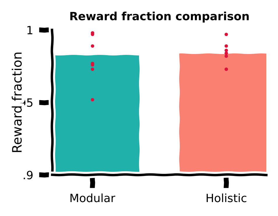
We first compute the fraction of rewarded trials in the total 1,000 trials for all training runs with different random seeds for the modular and holistic agents. We visualize this using a bar plot, with each red dot denoting the performance of a random seed.
Reward function comparison#
Show code cell source
# @title Reward function comparison

with plt.xkcd():
    xticks = [0, 1]; xticklabels = ['Modular', 'Holistic']
    yticks = [0.9, 0.95, 1]

    fig = plt.figure(figsize=(2.2, 1.7), dpi=200)
    ax = fig.add_subplot(1, 1, 1)
    ax.set_title('Reward fraction comparison', fontsize=fontsize, fontweight='bold')
    ax.spines['top'].set_visible(False); ax.spines['right'].set_visible(False)
    plt.xticks(xticks, xticklabels, fontsize=fontsize)
    plt.yticks(yticks, fontsize=fontsize)
    ax.set_xlabel(r'', fontsize=fontsize + 1)
    ax.set_ylabel('Reward fraction', fontsize=fontsize + 1)
    ax.set_xlim(xticks[0] - 0.3, xticks[-1] + 0.3)
    ax.set_ylim(yticks[0], yticks[-1])
    ax.xaxis.set_label_coords(0.5, -0.15)
    ax.yaxis.set_label_coords(-0.13, 0.5)
    ax.yaxis.set_major_formatter(major_formatter)

    for (idx, dfs), c in zip(enumerate([modular_dfs, holistic_dfs]), [modular_c, holistic_c]):
        ydata = [df.rewarded.sum() / len(df) for df in dfs]
        ax.bar(idx, np.mean(ydata), width=0.7, color=c, alpha=1, zorder=0)
        ax.scatter([idx] * len(ydata), ydata, c='crimson', marker='.',
                   s=10, lw=0.5, zorder=1, clip_on=False)

    fig.tight_layout(pad=0.1, rect=(0, 0, 1, 1))
Time spent comparison#
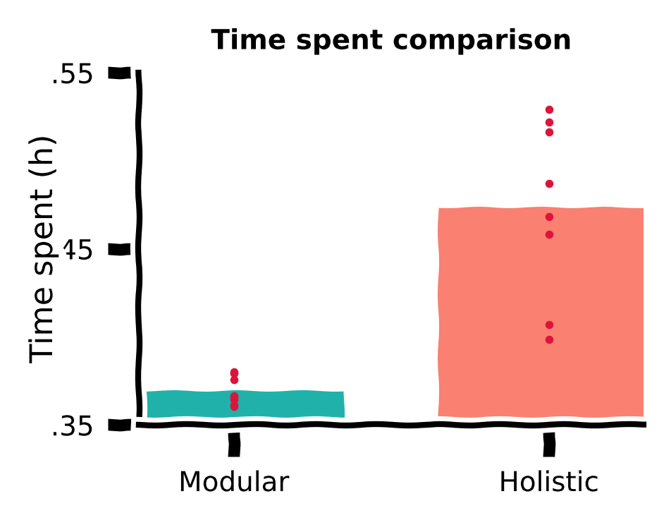
Despite similar performance measured by a rewarded fraction, we did observe qualitative differences in the trajectories of the two agents in the previous sections. It is possible that the holistic agent’s more curved trajectories, although reaching the target, are less efficient, i.e., they waste more time.
Therefore, we also plot the time spent by both agents for the same 1,000 targets.
Time spent comparison#
Show code cell source
# @title Time spent comparison

with plt.xkcd():
    xticks = [0, 1]; xticklabels = ['Modular', 'Holistic']
    yticks = [0.35, 0.45, 0.55]

    fig = plt.figure(figsize=(2.2, 1.7), dpi=200)
    ax = fig.add_subplot(1, 1, 1)
    ax.set_title('Time spent comparison', fontsize=fontsize, fontweight='bold')
    ax.spines['top'].set_visible(False); ax.spines['right'].set_visible(False)
    plt.xticks(xticks, xticklabels, fontsize=fontsize)
    plt.yticks(yticks, fontsize=fontsize)
    ax.set_xlabel(r'', fontsize=fontsize + 1)
    ax.set_ylabel('Time spent (h)', fontsize=fontsize + 1)
    ax.set_xlim(xticks[0] - 0.3, xticks[-1] + 0.3)
    ax.set_ylim(yticks[0], yticks[-1])
    ax.xaxis.set_label_coords(0.5, -0.15)
    ax.yaxis.set_label_coords(-0.16, 0.5)
    ax.yaxis.set_major_formatter(major_formatter)

    for (idx, dfs), c in zip(enumerate([modular_dfs, holistic_dfs]), [modular_c, holistic_c]):
        ydata = [(np.hstack(df.pos_x).size - len(df)) * arg.DT / 3600 for df in dfs]
        ax.bar(idx, np.mean(ydata), width=0.7, color=c, alpha=1, zorder=0)
        ax.scatter([idx] * len(ydata), ydata, c='crimson', marker='.',
                   s=10, lw=0.5, zorder=1, clip_on=False)

    fig.tight_layout(pad=0.1, rect=(0, 0, 1, 1))
Discussion#
Which agent’s behavior is more desired in the RL framework? Why?
Hint: Consider the objective functions for the critic and actor. The discount factor \(\gamma\) used in training is smaller than \(1\).
Training curve#
So far, we have only tested the agents after training. We can also visualize the performance curve for both agents during the training course.
During training, for every \(500\) training trials, the agent’s performance (fraction of rewarded trials) was evaluated. These data were saved; we’ll load them back in for visualization.
Load training curves#
Show code cell source
# @title Load training curves

training_curve_path = Path('training_curve')
holistic_curves = [pd.read_csv(file) for file in training_curve_path.glob(f'holistic*')]
modular_curves = [pd.read_csv(file) for file in training_curve_path.glob(f'modular*')]
Let us plot the training curves for both agents. The shaded area denotes the standard error of the mean across all random seeds.
Visualize training curves#
Show code cell source
# @title Visualize training curves

mean_holistic_curves = np.vstack([v.reward_fraction for v in holistic_curves]).mean(axis=0)
sem_holistic_curves = sem(np.vstack([v.reward_fraction for v in holistic_curves]), axis=0)
mean_modular_curves = np.vstack([v.reward_fraction for v in modular_curves]).mean(axis=0)
sem_modular_curves = sem(np.vstack([v.reward_fraction for v in holistic_curves]), axis=0)

xaxis_scale = int(1e4)
yticks = np.around(np.linspace(0, 1, 6), 1)
xticks = np.around(np.linspace(0, 1.5e5, 4), 1)
xticklabels = [my_tickformatter(i, None) for i in xticks / xaxis_scale]

with plt.xkcd():
    fig = plt.figure(figsize=(2.2, 1.7), dpi=200)
    ax = fig.add_subplot(1, 1, 1)
    ax.set_title('Reward fraction during training', fontsize=fontsize, fontweight='bold')
    ax.spines['top'].set_visible(False); ax.spines['right'].set_visible(False)
    plt.xticks(xticks, xticklabels, fontsize=fontsize)
    plt.yticks(yticks, fontsize=fontsize)
    ax.set_xlabel(r'Training trial ($\times$10$^4$)', fontsize=fontsize + 1)
    ax.set_ylabel('Reward fraction', fontsize=fontsize + 1)
    ax.set_xlim(xticks[0], xticks[-1])
    ax.set_ylim(yticks[0], yticks[-1])
    ax.xaxis.set_label_coords(0.5, -0.3)
    ax.yaxis.set_label_coords(-0.13, 0.5)
    ax.yaxis.set_major_formatter(major_formatter)

    xdata = holistic_curves[0].episode.values
    for ymean, ysem, color, label in zip([mean_holistic_curves, mean_modular_curves],
                                         [sem_holistic_curves, sem_modular_curves],
                                         [holistic_c, modular_c],
                                         ['Holistic agent', 'Modular agent']):
        ax.plot(xdata, ymean, lw=lw, clip_on=False, c=color, label=label)
        ax.fill_between(xdata, ymean - ysem, ymean + ysem, edgecolor='None',
                        facecolor=color, alpha=0.4, clip_on=True)

    ax.legend(fontsize=fontsize, frameon=False, loc=[0.26, 0.1],
              handletextpad=0.5, labelspacing=0.2, ncol=1, columnspacing=1)

    fig.tight_layout(pad=0.3, w_pad=0.5, rect=(0, 0, 1, 1))
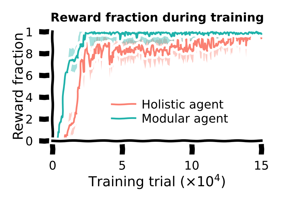
Conclusion for the training task: The modular agent learned faster and developed more efficient behaviors than the holistic agent.
Submit your feedback#
Show code cell source
# @title Submit your feedback
content_review(f"{feedback_prefix}_comparing_performance_of_agents")
Section 3: A novel gain task#
Estimated timing to here from start of tutorial: 50 minutes
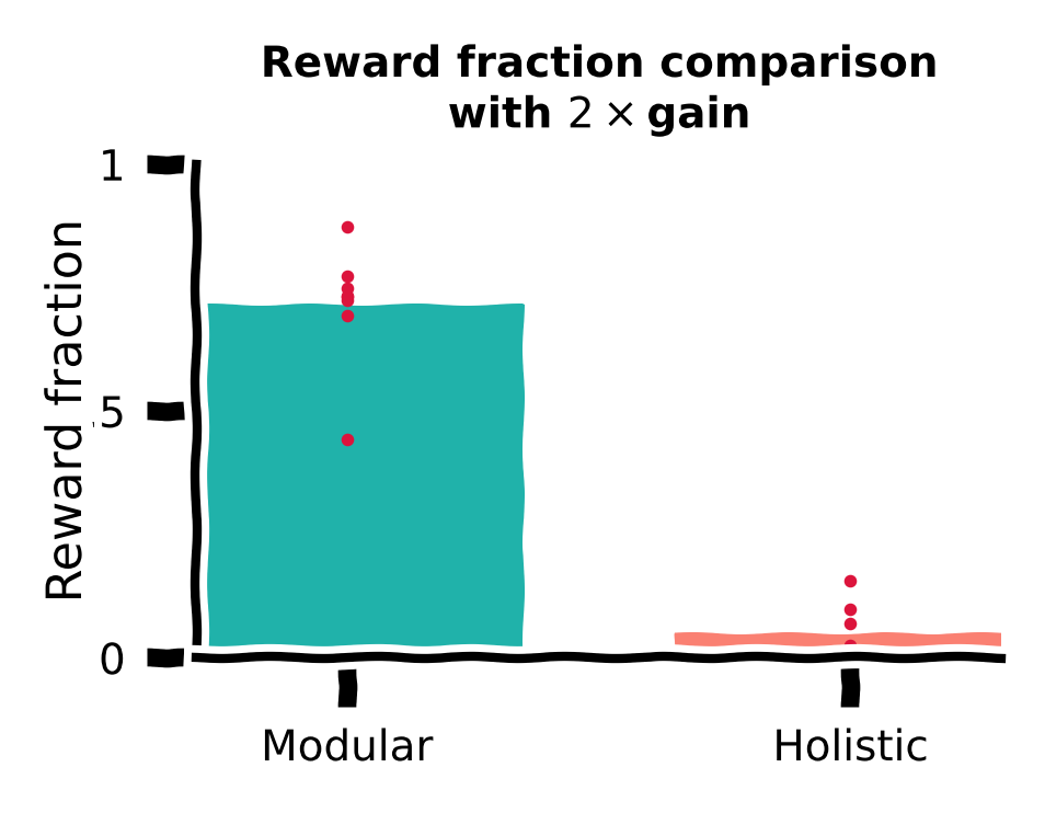
The prior task had a fixed joystick gain that meant consistent linear and angular velocities. We will now look at a novel task that tests the generalization capabilities of these models by varying this setting between training and testing. Will the model generalize well?
Video 7: Novel Task#
Submit your feedback#
Show code cell source
# @title Submit your feedback
content_review(f"{feedback_prefix}_novel_task_video")
A good architecture should not only learn fast but also generalize better.
One crucial parameter in our task is the joystick gain, which linearly maps motor actions (dimensionless, bounded in \([-1,1]\)) to corresponding velocities in the environment, i.e., velocity=gain \(\cdot\) action (see the environment dynamics above). During training, the gain remains fixed at \(200\) cm/s and \(90^{\circ}\)/s for linear and angular components, referred to as the \(1\times\) gain.
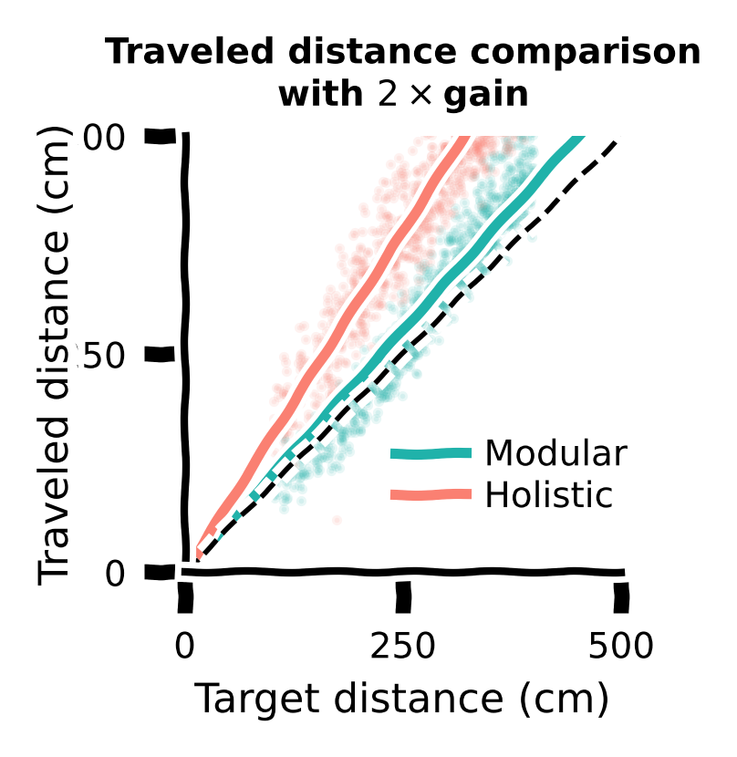
To test agents’ generalization abilities, here, we increase the gain to \(2\times\). This means the maximum velocities in the environment are doubled to \(400\) cm/s and \(180^{\circ}\)/s. Note that agents were only exposed to the \(1\times\) gain during training. Therefore, if they use the same sequence of actions as in training with the \(2\times\) gain, they will overshoot targets.
Let us evaluate modular and holistic agents with the same \(1000\) sampled targets again, but now with the \(2\times\) gain.

gain_factor = 2
Load holistic & modular agents#
Show code cell source
# @title Load holistic & modular agents
modular_agent = Agent(arg, ModularActor)
modular_agent.load(Path('agents/modular'), 0)
modular_dfs_2x = evaluation(modular_agent, gain_factor=gain_factor)

holistic_agent = Agent(arg, HolisticActor)
holistic_agent.load(Path('agents/holistic'), 0)
holistic_dfs_2x = evaluation(holistic_agent, gain_factor=gain_factor)
Let us first visualize the modular agents’ trajectories with \(2\times\) gain.
Modular agent’s trajectories#
Show code cell source
# @title Modular agent's trajectories

target_idexes = np.arange(0, 500)
df = modular_dfs_2x

fig = plt.figure(figsize=(2.2, 1.7), dpi=200)
ax = fig.add_subplot(111)
ax.set_title("Modular agent's trajectories\nwith " +
             r'$2\times$gain', fontsize=fontsize, fontweight='bold')
ax.set_aspect('equal')
ax.spines['top'].set_visible(False)
ax.spines['right'].set_visible(False)
ax.spines['bottom'].set_visible(False)
ax.spines['left'].set_visible(False)
ax.axes.xaxis.set_ticks([]); ax.axes.yaxis.set_ticks([])
ax.set_xlim([-235, 235]); ax.set_ylim([-2, 430])

ax.plot(np.linspace(0, 230 + 7), np.tan(np.deg2rad(55)) * np.linspace(0, 230 + 7) - 10,
        c='k', ls=(0, (1, 1)), lw=lw)
for _, trial in df.iloc[target_idexes].iterrows():
    ax.plot(trial.pos_x, trial.pos_y, c=modular_c, lw=0.3, ls='-', alpha=0.2)

reward_idexes = df.rewarded.iloc[target_idexes].values
for label, mask, c in zip(['Rewarded', 'Unrewarded'], [reward_idexes, ~reward_idexes],
                          [reward_c, unreward_c]):
    ax.scatter(*df.iloc[target_idexes].loc[mask, ['target_x', 'target_y']].values.T,
               c=c, marker='o', s=1, lw=1.5, label=label)

x_temp = np.linspace(-235, 235)
ax.plot(x_temp, np.sqrt(420**2 - x_temp**2), c='k', ls=(0, (1, 1)), lw=lw)
ax.text(-10, 425, s=r'70$\degree$', fontsize=fontsize)
ax.text(130, 150, s=r'400 cm', fontsize=fontsize)

ax.plot(np.linspace(-230, -130), np.linspace(0, 0), c='k', lw=lw)
ax.plot(np.linspace(-230, -230), np.linspace(0, 100), c='k', lw=lw)
ax.text(-230, 100, s=r'100 cm', fontsize=fontsize)
ax.text(-130, 0, s=r'100 cm', fontsize=fontsize)

ax.text(-210, 30, s="Modular agent's\ntrajectories", fontsize=fontsize - 0.5, c=modular_c)

ax.legend(fontsize=fontsize, frameon=False, loc=[0.56, 0.0],
          handletextpad=-0.5, labelspacing=0, ncol=1, columnspacing=1)

fig.tight_layout(pad=0)
Let us now visualize the holistic agents’ trajectories with \(2\times\) gain.
Holistic agent’s trajectories#
Show code cell source
# @title Holistic agent's trajectories

target_idexes = np.arange(0, 500)
df = holistic_dfs_2x

fig = plt.figure(figsize=(2.2, 1.7), dpi=200)
ax = fig.add_subplot(111)
ax.set_title("Holistic agent's trajectories\nwith " +
             r'$2\times$gain', fontsize=fontsize, fontweight='bold')
ax.set_aspect('equal')
ax.spines['top'].set_visible(False)
ax.spines['right'].set_visible(False)
ax.spines['bottom'].set_visible(False)
ax.spines['left'].set_visible(False)
ax.axes.xaxis.set_ticks([]); ax.axes.yaxis.set_ticks([])
ax.set_xlim([-235, 235]); ax.set_ylim([-2, 430])

ax.plot(np.linspace(0, 230 + 7), np.tan(np.deg2rad(55)) * np.linspace(0, 230 + 7) - 10,
        c='k', ls=(0, (1, 1)), lw=lw)
for _, trial in df.iloc[target_idexes].iterrows():
    ax.plot(trial.pos_x, trial.pos_y, c=holistic_c, lw=0.3, ls='-', alpha=0.2)

reward_idexes = df.rewarded.iloc[target_idexes].values
for label, mask, c in zip(['Rewarded', 'Unrewarded'], [reward_idexes, ~reward_idexes],
                          [reward_c, unreward_c]):
    ax.scatter(*df.iloc[target_idexes].loc[mask, ['target_x', 'target_y']].values.T,
               c=c, marker='o', s=1, lw=1.5, label=label)


x_temp = np.linspace(-235, 235)
ax.plot(x_temp, np.sqrt(420**2 - x_temp**2), c='k', ls=(0, (1, 1)), lw=lw)
ax.text(-10, 425, s=r'70$\degree$', fontsize=fontsize)
ax.text(130, 150, s=r'400 cm', fontsize=fontsize)

ax.plot(np.linspace(-230, -130), np.linspace(0, 0), c='k', lw=lw)
ax.plot(np.linspace(-230, -230), np.linspace(0, 100), c='k', lw=lw)
ax.text(-230, 100, s=r'100 cm', fontsize=fontsize)
ax.text(-130, 0, s=r'100 cm', fontsize=fontsize)

ax.text(-210, 30, s="Holistic agent's\ntrajectories", fontsize=fontsize - 0.5, c=holistic_c)

ax.legend(fontsize=fontsize, frameon=False, loc=[0.56, 0.0],
          handletextpad=-0.5, labelspacing=0, ncol=1, columnspacing=1)

fig.tight_layout(pad=0)
Discussion#
Do the two agents have the same generalization abilities?
Again, let us load the saved evaluation data with the \(2\times\) gain for agents with all \(8\) random seeds.
Load data#
Show code cell source
# @title Load data
with open('modular_dfs_2x.pkl', 'rb') as file:
    modular_dfs_2x = pickle.load(file)

with open('holistic_dfs_2x.pkl', 'rb') as file:
    holistic_dfs_2x = pickle.load(file)
Now, let’s compare reward fraction with \(2\times\) gain.
Reward function comparison#
Show code cell source
# @title Reward function comparison

with plt.xkcd():
    xticks = [0, 1]; xticklabels = ['Modular', 'Holistic']
    yticks = [0, 0.5, 1]

    fig = plt.figure(figsize=(2.2, 1.7), dpi=200)
    ax = fig.add_subplot(111)
    ax.set_title("Reward fraction comparison\nwith " +
                 r'$2\times$gain', fontsize=fontsize, fontweight='bold')
    ax.spines['top'].set_visible(False); ax.spines['right'].set_visible(False)
    plt.xticks(xticks, xticklabels, fontsize=fontsize)
    plt.yticks(yticks, fontsize=fontsize)
    ax.set_xlabel(r'', fontsize=fontsize + 1)
    ax.set_ylabel('Reward fraction', fontsize=fontsize + 1)
    ax.set_xlim(xticks[0] - 0.3, xticks[-1] + 0.3)
    ax.set_ylim(yticks[0], yticks[-1])
    ax.xaxis.set_label_coords(0.5, -0.15)
    ax.yaxis.set_label_coords(-0.13, 0.5)
    ax.yaxis.set_major_formatter(major_formatter)

    for (idx, dfs), c in zip(enumerate([modular_dfs_2x, holistic_dfs_2x]), [modular_c, holistic_c]):
        ydata = [df.rewarded.sum() / len(df) for df in dfs]
        ax.bar(idx, np.mean(ydata), width=0.7, color=c, alpha=1, zorder=0)
        ax.scatter([idx] * len(ydata), ydata, c='crimson', marker='.',
                   s=10, lw=0.5, zorder=1, clip_on=False)

    fig.tight_layout(pad=0.1, rect=(0, 0, 1, 1))
Let us also compare traveled distance vs target distance with \(2\times\) gain for different agents.
Traveled distance comparison#
Show code cell source
# @title Traveled distance comparison
with plt.xkcd():
    xticks = np.array([0, 250, 500])
    yticks = xticks

    fig = plt.figure(figsize=(2, 2), dpi=200)
    ax = fig.add_subplot(111)
    ax.set_title("Traveled distance comparison\nwith " +
                 r'$2\times$gain', fontsize=fontsize, fontweight='bold')
    ax.set_aspect('equal')
    ax.spines['top'].set_visible(False); ax.spines['right'].set_visible(False)
    plt.xticks(xticks, fontsize=fontsize)
    plt.yticks(yticks, fontsize=fontsize)
    ax.set_xlabel('Target distance (cm)', fontsize=fontsize + 1)
    ax.set_ylabel('Traveled distance (cm)', fontsize=fontsize + 1)
    ax.set_xlim(xticks[0], xticks[-1])
    ax.set_ylim(yticks[0], yticks[-1])
    ax.xaxis.set_label_coords(0.5, -0.25)
    ax.yaxis.set_label_coords(-0.25, 0.5)
    ax.yaxis.set_major_formatter(major_formatter)

    xdata_m = np.hstack([df.target_r for df in modular_dfs_2x])
    ydata_m = np.hstack([df.pos_r_end for df in modular_dfs_2x])
    xdata_h = np.hstack([df.target_r for df in holistic_dfs_2x])
    ydata_h = np.hstack([df.pos_r_end for df in holistic_dfs_2x])

    sampled_trial_idx = np.random.choice(np.arange(ydata_m.size), size=1000, replace=False)

    ax.scatter(xdata_m[sampled_trial_idx], ydata_m[sampled_trial_idx], c=modular_c, s=1, alpha=0.1)
    ax.scatter(xdata_h[sampled_trial_idx], ydata_h[sampled_trial_idx], c=holistic_c, s=1, alpha=0.1)

    model = LinearRegression(fit_intercept=False)
    model.fit(xdata_m.reshape(-1, 1), ydata_m)
    ax.plot(xticks, model.predict(xticks.reshape(-1, 1)), c=modular_c,
            ls='-', lw=lw*2, label='Modular')

    model = LinearRegression(fit_intercept=False)
    model.fit(xdata_h.reshape(-1, 1), ydata_h)
    ax.plot(xticks, model.predict(xticks.reshape(-1, 1)), c=holistic_c,
            ls='-', lw=lw*2, label='Holistic')

    ax.plot(xticks, yticks, c='k', ls='--', lw=lw)

    ax.legend(fontsize=fontsize, frameon=False, loc=[0.45, 0.1],
              handletextpad=0.5, labelspacing=0.2, ncol=1, columnspacing=1)

    fig.tight_layout(pad=0.1, rect=(0, 0, 1, 1))
Discussion:#
What have you found? Which agent generalized better?
Submit your feedback#
Show code cell source
# @title Submit your feedback
content_review(f"{feedback_prefix}_novel_gain_task")
Decoding analysis#
Although we have confirmed that the modular agent exhibited better generalization performance in the gain task, the underlying mechanism remains unclear. One reasonable hypothesis is that the modular agent has a robust belief that remains accurate with the \(2\times\) gain. Therefore, this robust belief can support good actions. Ultimately, agents should be aware of its location to avoid overshooting.
To test this hypothesis, we recorded the activities of RNN neurons in the agents’ actors, as these neurons are responsible for computing the beliefs underlying actions. Since beliefs should represent the agents’ locations in the environment, we used linear regression (with \(\ell_2\) regularization) to decode agents’ locations from the recorded RNN activities.
We defined the decoding error, representing the Euclidean distance between the true and decoded locations, as an indicator of belief accuracy.
Load data#
Show code cell source
# @title Load data
modular_decoder_data = [fit_decoder(df) for df in modular_dfs]
modular_decoder_data_2x = [fit_decoder(df) for df in modular_dfs_2x]
modular_decoding_error = np.hstack([np.linalg.norm(v[2] - v[0].predict(v[1]), axis=1) for v
                                    in modular_decoder_data])
modular_decoding_error_2x = np.hstack([np.linalg.norm(v[2] - v[0].predict(v[1]), axis=1) for v
                                       in modular_decoder_data_2x])

holistic_decoder_data = [fit_decoder(df) for df in holistic_dfs]
holistic_decoder_data_2x = [fit_decoder(df) for df in holistic_dfs_2x]
holistic_decoding_error = np.hstack([np.linalg.norm(v[2] - v[0].predict(v[1]), axis=1) for v
                                     in holistic_decoder_data])
holistic_decoding_error_2x = np.hstack([np.linalg.norm(v[2] - v[0].predict(v[1]), axis=1) for v
                                        in holistic_decoder_data_2x])
We plot the distribution of the decoding error for every step in every trial across random seeds for each agent, under \(1×\) or \(2×\) gain.
Decoding error comparison#
Show code cell source
# @title Decoding error comparison

with plt.xkcd():
    xticks = np.array([0, 1]); xticklabels = ['1x (train)', '2x (test)']
    yticks = np.linspace(0, 120, 5)

    fig = plt.figure(figsize=(2.2, 1.7), dpi=200)
    ax = fig.add_subplot(111)
    ax.set_title('Decoding error comparison', fontsize=fontsize, fontweight='bold')
    ax.spines['top'].set_visible(False); ax.spines['right'].set_visible(False)
    plt.xticks(xticks, xticklabels, fontsize=fontsize)
    plt.yticks(yticks, fontsize=fontsize)
    ax.set_xlabel(r'Gain', fontsize=fontsize + 1)
    ax.set_ylabel('Decoding error (cm)', fontsize=fontsize + 1)
    ax.set_xlim(xticks[0] - 0.2, xticks[-1] + 0.2)
    ax.set_ylim(yticks[0], yticks[-1])
    ax.xaxis.set_label_coords(0.5, -0.15)
    ax.yaxis.set_label_coords(-0.2, 0.5)
    ax.yaxis.set_major_formatter(major_formatter)

    violin1 = ax.violinplot(filter_fliers([modular_decoding_error, modular_decoding_error_2x]),
                            positions=xticks - 0.1, showmeans=True, widths=0.1)
    set_violin_plot(violin1, facecolor=modular_c, edgecolor=modular_c)

    violin2 = ax.violinplot(filter_fliers([holistic_decoding_error, holistic_decoding_error_2x]),
                            positions=xticks + 0.1, showmeans=True, widths=0.1)
    set_violin_plot(violin2, facecolor=holistic_c, edgecolor=holistic_c)

    ax.legend([violin1['bodies'][0], violin2['bodies'][0]], ['Modular', 'Holistic'],
              fontsize=fontsize, frameon=False, loc=[0.3, 0.7],
              handletextpad=0.5, labelspacing=0.2, ncol=1, columnspacing=1)

    fig.tight_layout(pad=0.1, rect=(0, 0, 1, 1))
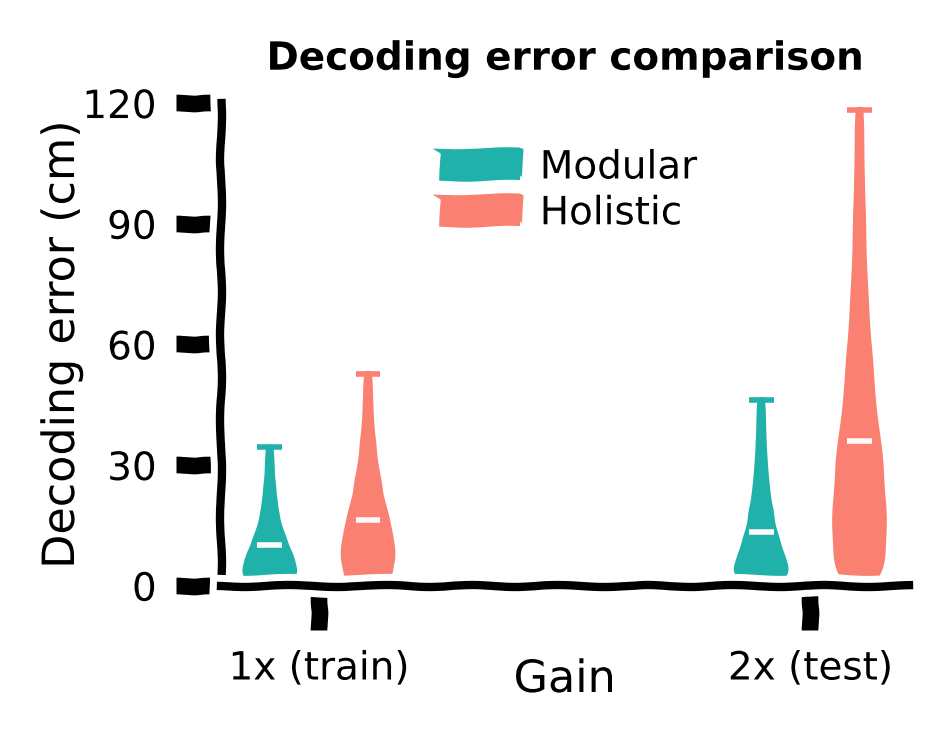
While both agents demonstrated small decoding errors with the training gain, we observed that the holistic agent, which struggled with generalization at the \(2×\) gain, also exhibited reduced accuracy in determining its own location. This helps explain why the modular agent can generalize better at higher gains.
Conclusion for the gain task: In the gain task, the modular agent exhibited better generalization than the holistic agent, supported by a more accurate internal belief when faced with larger gains.
Submit your feedback#
Show code cell source
# @title Submit your feedback
content_review(f"{feedback_prefix}_decoding_analysis")
The Big Picture#
Estimated timing of tutorial: 1 hour
In this tutorial, we explored the difference in agents’ performance based on their architecture. We revealed that modular architecture, with separate modules for learning different aspects of behavior, is superior to a holistic architecture with a single module. The modular architecture with stronger inductive bias achieves good performance faster and has the capability to generalize to other tasks as well. Intriguingly, this modularity is a property we also observe in the brains, which could be important for generalization in the brain as well.
Addendum: Generalization, but no free lunch#
The No Free Lunch theorems proved that no inductive bias can excel across all tasks. It has been studied in the paper that agents with a modular architecture can acquire the underlying structure of the training task. In contrast, holistic agents tend to acquire different knowledge than modular agents during training, such as forming beliefs based on unreliable information sources or exhibiting less efficient control actions. The novel gain task has a structure similar to the training task, consequently, a modular agent that accurately learns the training task’s structure can leverage its knowledge in these novel tasks.
However, it is worth noting that an infinite number of new tasks can be constructed, diverging from the training task’s structure but aligning with the ‘inferior’ beliefs and control acquired by holistic agents.
For example, although we have seen that the holistic agent developed inefficient trajectories with higher curvature, which is detrimental for the training task, if we consider a new task with a different reward function, such as preferring more curved trajectories, the holistic agent should perform better in this particular task than the modular agent. There is no free lunch.
Submit your feedback#
Show code cell source
# @title Submit your feedback
content_review(f"{feedback_prefix}_generalization_but_no_free_lunch")


