Tutorial 3: Statistical inference on representational geometries

Tutorial 3: Statistical inference on representational geometries#

Week 1, Day 3: Comparing Artificial And Biological Networks

By Neuromatch Academy

Content creators: Veronica Bossio, Eivinas Butkus, Jasper van den Bosch

Content reviewers: Samuele Bolotta, Yizhou Chen, RyeongKyung Yoon, Ruiyi Zhang, Lily Chamakura, Patrick Mineault, Hlib Solodzhuk

Production editors: Konstantine Tsafatinos, Ella Batty, Spiros Chavlis, Samuele Bolotta, Hlib Solodzhuk, Patrick Mineault

Tutorial Objectives#

Estimated timing of tutorial: 50 minutes

To evaluate alternative models of measured data, we need statistical inference that takes our uncertainty about relative model performance into account. In computational neuroscience, we want to statistically compare different models in terms of their ability to account for representations in brains. In AI, we can employ similar techniques to compare models to each other and understand their internal representations.

By the end of this tutorial, you will be able to:

Understand Representational Similarity Analysis (RSA), including its theoretical foundations, practical applications, and its significance in the context of machine learning and computational neuroscience.
Extract neural network activations; understand the structure of neural networks, the role of activations in interpreting neural network decisions, and practical techniques for accessing these activations.
Discuss frequentist model comparison: This part of the tutorial will cover the basics of frequentist model comparison methods. It will provide an overview of the principles underlying these methods and their applications.
Identify sources of estimation error and the motivation for model-comparative frequentist inference. You will learn about the three main sources of estimation error in statistical inference—measurement noise, stimulus sampling, and subject sampling. Additionally, the tutorial will explore how these sources of error justify the use of model-comparative frequentist inference, particularly through the application of the 2-factor bootstrap method. This section will detail the impact of each source of error on statistical inference and demonstrate how the 2-factor bootstrap accounts for our uncertainty about model performance during model comparison.

Setup#

Install and import feedback gadget#

Import dependencies#

Figure settings#

Plotting functions#

Show code cell source Hide code cell source

# @title Plotting functions

def traces_bar_and_scatter(eval_result, models, bar_color='blue'):

    evaluations = eval_result.evaluations.squeeze()
    subject_names = [f'Subject {i+1}' for i in range(evaluations.shape[1])]
    model_names = [model.name for model in models]
    df_evaluations = pd.DataFrame(data=evaluations, index=model_names, columns=subject_names)
    means = df_evaluations.mean(axis=1)
    sem = df_evaluations.sem(axis=1)

    bars_trace = go.Bar(
        x=model_names,
        y=means,
        showlegend=False,
        marker_color=bar_color
    )

    scatter_traces = []
    for subject in subject_names:
        if subject == "Subject 1":
            showlegend = True
        scatter_traces.append(go.Scatter(
            x=df_evaluations.index,
            y=df_evaluations[subject],
            mode='markers',
            marker=dict(size=5,
                        color='white',
                        line=dict(width=1)),
            showlegend=False
        ))
    blank_trace = go.Scatter(
        x=[None],  # This ensures the trace doesn't actually plot data
        y=[None],
        mode='markers',
        marker=dict(size=5, color='white', line=dict(width=1)),
        name='Each dot represents <br> a subject'
        )
    return bars_trace, scatter_traces, blank_trace

def plot_bars_and_scatter_from_trace(bars_trace, scatter_traces, blank_trace):

    fig = go.Figure()
    fig.add_trace(bars_trace)
    for trace in scatter_traces:
        fig.add_trace(trace)
    fig.add_trace(blank_trace)
    fig.update_layout(
        title="",
        xaxis_title="Model",
        yaxis_title="Cosine Similarity to Data RDMs",
        legend_title="",
        width=700,
        height=500,
        template="simple_white"
    )
    return fig

def convert_result_to_list_of_dicts(result):
    means = result.get_means()
    sems = result.get_sem()
    p_zero = result.test_zero()
    p_noise = result.test_noise()
    model_names = [model.name for model in result.models]

    results_list = []
    for i, model_name in enumerate(model_names):
        result_dict = {
            "Model": model_name,
            "Eval±SEM": f"{means[i]:.3f} ± {sems[i]:.3f}",
            "p (against 0)": "< 0.001" if p_zero[i] < 0.001 else f"{p_zero[i]:.3f}",
            "p (against NC)": "< 0.001" if p_noise[i] < 0.001 else f"{p_noise[i]:.3f}"
        }
        results_list.append(result_dict)

    return results_list

def print_results_table(table_trace):

    fig = go.Figure()
    fig.add_trace(table_trace)

    return fig

def get_trace_for_table(eval_result):

    results_list = convert_result_to_list_of_dicts(eval_result)

    table_trace = go.Table(
        header=dict(values=["Model", "Eval ± SEM", "p (against 0)", "p (against NC)"]),
        cells=dict(
            values=[
                [result["Model"] for result in results_list],  # Correctly accesses each model name
                [result["Eval±SEM"] for result in results_list],  # Correctly accesses the combined Eval and SEM value
                [result["p (against 0)"] for result in results_list],  # Accesses p-value against 0
                [result["p (against NC)"] for result in results_list]  # Accesses p-value against noise ceiling
            ],
            font=dict(size=12),  # Smaller font size for the cells
            height=27  # Smaller height for the cell rows
            )
    )
    return table_trace

def get_trace_for_noise_ceiling(noise_ceiling):

    noise_lower = np.nanmean(noise_ceiling[0])
    noise_upper = np.nanmean(noise_ceiling[1])
    #model_names = [model.name for model in models]

    noise_rectangle = dict(
            # Rectangle reference to the axes
            type="rect",
            xref="x domain",  # Use 'x domain' to span the whole x-axis
            yref="y",  # Use specific y-values for the height
            x0=0,  # Starting at the first x-axis value
            y0=noise_lower,  # Bottom of the rectangle
            x1=1,  # Ending at the last x-axis value (in normalized domain coordinates)
            y1=noise_upper,  # Top of the rectangle
            fillcolor="rgba(128, 128, 128, 0.4)",  # Light grey fill with some transparency
            line=dict(
                width=0,
                #color="rgba(128, 128, 128, 0.5)",
            )

        )
    return noise_rectangle

def plot_bars_and_scatter_with_table(eval_result, models, method, color='blue', table = True):

    if method == 'cosine':
         method_name = 'Cosine Similarity'
    elif method == 'corr':
        method_name = 'Correlation distance'
    else:
        method_name = 'Comparison method?'

    if table:
        cols = 2
        subplot_titles=["Model Evaluations", "Model Statistics"]
    else:
        cols = 1
        subplot_titles=["Model Evaluations"]

    fig = make_subplots(rows=1, cols=cols,
                        #column_widths=[0.4, 0.6],
                        subplot_titles=subplot_titles,
                        #specs=[[{"type": "bar"}, {"type": "table"}]]

                            )

    bars_trace, scatter_traces, blank_trace = traces_bar_and_scatter(eval_result, models, bar_color=color)

    fig.add_trace(bars_trace, row=1, col=1)

    for trace in scatter_traces:
        fig.add_trace(trace, row=1, col=1)

    if table:
        table_trace = get_trace_for_table(eval_result)
        fig.add_trace(table_trace, row=1, col=2)

    width = 600*cols

    fig.update_layout(
        yaxis_title=f"RDM prediction accuracy <br> (across subject mean of {method_name})",
        #legend_title="",
        width=width,
        height=600,
        template="plotly_white"
    )

    return fig

def add_noise_ceiling_to_plot(fig, noise_ceiling):

        rectangle = get_trace_for_noise_ceiling(noise_ceiling)
        fig.add_shape(rectangle, row=1, col=1)
        return fig


def bar_bootstrap_interactive(human_rdms, models_to_compare, method):

    color = 'orange'

    button = widgets.Button(
    description="New Bootstrap Sample",
    layout=widgets.Layout(width='auto', height='auto')  # Adjust width and height as needed
    )

    #button.style.button_color = 'lightblue'  # Change the button color as you like
    button.style.font_weight = 'bold'
    button.layout.width = '300px'  # Make the button wider
    button.layout.height = '48px'  # Increase the height for a squarer appearance
    button.layout.margin = '0 0 0 0'  # Adjust margins as needed
    button.layout.border_radius = '12px'  # Rounded corners for the button

    output = widgets.Output(layout={'border': '1px solid black'})

    def generate_plot(bootstrap=False):
        if bootstrap:
                boot_rdms, idx = bootstrap_sample_rdm(human_rdms, rdm_descriptor='subject')
                result = eval.eval_fixed(models_to_compare, boot_rdms, method=method)
        else:
                result = eval.eval_fixed(models_to_compare, human_rdms, method=method)

        with output:
            clear_output(wait=True)  # Make sure to clear previous output first

            fig = plot_bars_and_scatter_with_table(result, models_to_compare, method, color)
            fig.update_layout(height=600, width=1150,
                              title=dict(text = f"Performance of Model layers for a random bootstrap sample of subjects",
                              x=0.5, y=0.95,
                              font=dict(size=20)))
            fig.show()  # Display the figure within the `with` context


    def on_button_clicked(b):
        generate_plot(bootstrap=True)

    # Now, let's create a VBox to arrange the button above the output
    vbox_layout = widgets.Layout(
        display='flex',
        flex_flow='column',
        align_items='stretch',
        width='100%',
    )


    output = widgets.Output(layout={'border': '1px solid black'})
    button.on_click(lambda b: generate_plot(bootstrap=True))  # Generate plot on button click
    vbox = widgets.VBox([button, output], layout=vbox_layout)

    # Display everything
    display(button, output)

    generate_plot(bootstrap=False)

def show_rdm_plotly(rdms, pattern_descriptor=None, cmap='Greys',
                    rdm_descriptor=None, n_column=None, n_row=None,
                    show_colorbar=False, gridlines=None, figsize=(None, None),
                    vmin=None, vmax=None):
    # Determine the number of matrices
    mats = rdms.get_matrices()
    n_matrices = mats.shape[0]


    # Determine the number of subplots
    if n_row is None or n_column is None:
        # Calculate rows and columns to fit all matrices in a roughly square layout
        n_row = 1
        n_column = n_matrices

        # n_side = int(n_matrices ** 0.5)
        # n_row = n_side if n_side ** 2 >= n_matrices else n_side + 1
        # n_column = n_row if n_row * (n_row - 1) < n_matrices else n_row - 1

    subplot_size = 150
    fig_width = n_column * subplot_size
    fig_height = n_row * subplot_size
    subplot_titles = [f'{rdm_descriptor } {rdms.rdm_descriptors[rdm_descriptor][i]}' for i in range(n_matrices)] if rdm_descriptor else None
    # Create subplots
    fig = make_subplots(rows=n_row, cols=n_column,
                        subplot_titles=subplot_titles,
                        shared_xaxes=True, shared_yaxes=True,
                        horizontal_spacing=0.02, vertical_spacing=0.1)

    # Iterate over RDMs and add them as heatmaps
    for index in range(n_matrices):
        row, col = divmod(index, n_column)
        fig.add_trace(
            go.Heatmap(z=mats[index],
                       colorscale=cmap,
                       showscale=show_colorbar,
                       zmin=vmin, zmax=vmax),
            row=row+1, col=col+1
        )

    fig.update_layout(height=290, width=fig_width)
    fig.update_xaxes(showticklabels=False)
    fig.update_yaxes(showticklabels=False)


    #fig.show()
    return fig

def show_rdm_plotly_interactive_bootstrap_patterns(rdms, pattern_descriptor=None, cmap='Greys',
                    rdm_descriptor=None, n_column=None, n_row=None,
                    show_colorbar=False, gridlines=None, figsize=(None, None),
                    vmin=None, vmax=None):


    button = widgets.Button(
    description="New Bootstrap Sample",
    layout=widgets.Layout(width='auto', height='auto')  # Adjust width and height as needed
    )

    #button.style.button_color = 'lightblue'  # Change the button color as you like
    button.style.font_weight = 'bold'
    button.layout.width = '300px'  # Make the button wider
    button.layout.height = '48px'  # Increase the height for a squarer appearance
    button.layout.margin = '0 0 0 0'  # Adjust margins as needed
    button.layout.border_radius = '12px'  # Rounded corners for the button

    #output = widgets.Output(layout={'border': '1px solid black'})
    output = widgets.Output()

    def generate_plot(bootstrap=False):
        if bootstrap:
                im_boot_rdms, pattern_idx = bootstrap_sample_pattern(rdms, pattern_descriptor='index')
        else:
                im_boot_rdms = rdms

        with output:
            clear_output(wait=True)  # Make sure to clear previous output first

            fig = show_rdm_plotly(im_boot_rdms.subset('roi', 'FFA'), rdm_descriptor='subject')
            fig.update_layout(title=dict(text = f"Bootstrapped sample of patterns",
                                    x=0.5, y=0.95,
                                    font=dict(size=20)))
            fig.show()

    def on_button_clicked(b):
        generate_plot(bootstrap=True)

    # Now, let's create a VBox to arrange the button above the output
    vbox_layout = widgets.Layout(
        display='flex',
        flex_flow='column',
        align_items='stretch',
        width='100%',
    )

    button.on_click(lambda b: generate_plot(bootstrap=True))  # Generate plot on button click
    vbox = widgets.VBox([button, output], layout=vbox_layout)

    display(vbox)

    generate_plot(bootstrap=False)

def plot_model_comparison_trans(result, sort=False, colors=None,
                          alpha=0.01, test_pair_comparisons=True,
                          multiple_pair_testing='fdr',
                          test_above_0=True,
                          test_below_noise_ceil=True,
                          error_bars='sem',
                          test_type='t-test'):


    # Prepare and sort data
    evaluations = result.evaluations
    models = result.models
    noise_ceiling = result.noise_ceiling
    method = result.method
    model_var = result.model_var
    diff_var = result.diff_var
    noise_ceil_var = result.noise_ceil_var
    dof = result.dof

    while len(evaluations.shape) > 2:
        evaluations = np.nanmean(evaluations, axis=-1)

    evaluations = evaluations[~np.isnan(evaluations[:, 0])]
    n_bootstraps, n_models = evaluations.shape
    perf = np.mean(evaluations, axis=0)

    noise_ceiling = np.array(noise_ceiling)
    sort = 'unsorted'
    # run tests
    if any([test_pair_comparisons,
            test_above_0, test_below_noise_ceil]):
        p_pairwise, p_zero, p_noise = all_tests(
            evaluations, noise_ceiling, test_type,
            model_var=model_var, diff_var=diff_var,
            noise_ceil_var=noise_ceil_var, dof=dof)

    if error_bars:
        limits = get_errorbars(model_var, evaluations, dof, error_bars,
                               test_type)
        if error_bars.lower() == 'sem':
            limits = limits[0,:]

    #return limits, perf

    fig = make_subplots(rows=2, cols=1,
                        row_heights=[0.3, 0.7],
                        vertical_spacing=0.05,
                        subplot_titles=("Model Evaluations", ''),
                        shared_xaxes=True,
                        )

    n_colors_needed = len(models)
    # Sample n_colors_needed colors from the Plasma color scale
    plasma_scale = plotly.colors.get_colorscale('Bluered')  # Retrieve the color scale
    color_indices = np.linspace(0, 1, n_colors_needed)  # Evenly spaced indices between 0 and 1
    sampled_colors = plotly.colors.sample_colorscale(plasma_scale, color_indices)  # Sample colors

    for i, (perf_val, model) in enumerate(zip(perf, models)):
        name = model.name
        #bar_color = antique_colors[i % n_colors]

        fig.add_trace(
            go.Bar(
                x=[name],  # x-axis position
                y=[perf_val],  # Performance value
                error_y=dict(type='data',
                            array=limits, visible=True, color='black'),  # Adding error bars
                marker_color=sampled_colors[i],  # Cycle through colors
                name=name
            ),
            row=2, col=1  # Assuming a single subplot for simplicity
        )


    fig.update_layout(width=600, height=700, showlegend=False, template='plotly_white')
    # return fig


    model_significant = p_zero < alpha / n_models
    significant_indices = [i for i, significant in enumerate(model_significant) if significant]
    symbols = {'dewdrops': 'circle', 'icicles': 'diamond-tall'}

    fig.add_trace(
        go.Scatter(
            x=[models[i].name for i in significant_indices],  # X positions of significant models
            y=[0.0005] * len(significant_indices),  # Y positions (at 0 for visualization)
            mode='markers',
            marker=dict(symbol=symbols['dewdrops'],  # Example using 'triangle-up'
                        size=9,
                        color='white'),  # Example using 'triangle-up'
            showlegend=False
        ),
        row=2, col=1
    )

    # Plot noise ceiling
    if noise_ceiling is not None:

        noise_lower = np.nanmean(noise_ceiling[0])
        noise_upper = np.nanmean(noise_ceiling[1])
        model_names = [model.name for model in models]

        fig.add_shape(
                # Rectangle reference to the axes
                type="rect",
                xref="x domain",  # Use 'x domain' to span the whole x-axis
                yref="y",  # Use specific y-values for the height
                x0=0,  # Starting at the first x-axis value
                y0=noise_lower,  # Bottom of the rectangle
                x1=1,  # Ending at the last x-axis value (in normalized domain coordinates)
                y1=noise_upper,  # Top of the rectangle
                fillcolor="rgba(128, 128, 128, 0.5)",  # Light grey fill with some transparency
                line=dict(
                    color='gray',
                ),
                opacity=0.5,
                layer="below",  # Ensure the shape is below the data points
                row=2, col=1  # Specify the subplot where the shape should be added

            )

    test_below_noise_ceil = 'dewdrops'  # Example, can be True/'dewdrops'/'icicles'
    model_below_lower_bound = p_noise < (alpha / n_models)

    significant_indices_below = [i for i, below in enumerate(model_below_lower_bound) if below]

    # Choose the symbol based on the test_below_noise_ceil
    if test_below_noise_ceil is True or test_below_noise_ceil.lower() == 'dewdrops':
        symbol = 'circle-open'  # Use open circle as a proxy for dewdrops
    elif test_below_noise_ceil.lower() == 'icicles':
        symbol = 'diamond-open'  # Use open diamond as a proxy for icicles
    else:
        raise ValueError('Argument test_below_noise_ceil is incorrectly defined as ' + test_below_noise_ceil)

    symbol = 'triangle-down'
#    y_position_below = noise_lower + 0.0005  # Adjust based on your visualization needs

    #y_positions_below = [perf[i] for i in significant_indices_below]  # Extracting perf values for significant models
    y_positions_below = [noise_lower-0.005] * len(significant_indices_below)  # Adjust based on your visualization needs
    fig.add_trace(
        go.Scatter(
            x=[models[i].name for i in significant_indices_below],  # X positions of significant models
            y= y_positions_below, #* len(significant_indices_below),  # Y positions slightly above noise_lower
            mode='markers',
            marker=dict(symbol=symbol, size=7, color='gray'),  # Customizing marker appearance
            showlegend=False
        ),
        row=2, col=1
    )

    # Pairwise model comparisons
    if test_pair_comparisons:
        if test_type == 'bootstrap':
            model_comp_descr = 'Model comparisons: two-tailed bootstrap, '
        elif test_type == 't-test':
            model_comp_descr = 'Model comparisons: two-tailed t-test, '
        elif test_type == 'ranksum':
            model_comp_descr = 'Model comparisons: two-tailed Wilcoxon-test, '
        n_tests = int((n_models ** 2 - n_models) / 2)
        if multiple_pair_testing is None:
            multiple_pair_testing = 'uncorrected'
        if multiple_pair_testing.lower() == 'bonferroni' or \
           multiple_pair_testing.lower() == 'fwer':
            significant = p_pairwise < (alpha / n_tests)
        elif multiple_pair_testing.lower() == 'fdr':
            ps = batch_to_vectors(np.array([p_pairwise]))[0][0]
            ps = np.sort(ps)
            criterion = alpha * (np.arange(ps.shape[0]) + 1) / ps.shape[0]
            k_ok = ps < criterion
            if np.any(k_ok):
                k_max = np.max(np.where(ps < criterion)[0])
                crit = criterion[k_max]
            else:
                crit = 0
            significant = p_pairwise < crit
        else:
            if 'uncorrected' not in multiple_pair_testing.lower():
                raise ValueError(
                    'plot_model_comparison: Argument ' +
                    'multiple_pair_testing is incorrectly defined as ' +
                    multiple_pair_testing + '.')
            significant = p_pairwise < alpha
        model_comp_descr = _get_model_comp_descr(
            test_type, n_models, multiple_pair_testing, alpha,
            n_bootstraps, result.cv_method, error_bars,
            test_above_0, test_below_noise_ceil)


        # new_fig_nili = plot_nili_bars_plotly(fig, significant, models, version=1)
        # new_fig_gol = plot_golan_wings_plotly(fig, significant, perf, models)

        new_fig_metro = plot_metroplot_plotly(fig, significant, perf, models, sampled_colors)

        return new_fig_metro

def plot_golan_wings_plotly(original_fig, significant, perf, models):
    with plt.xkcd():
        # First, create a deep copy of the original figure to preserve its state
        fig = deepcopy(original_fig)

        n_models = len(models)
        model_names = [m.name for m in models]
        # Use the Plotly qualitative color palette
        colors = plotly.colors.qualitative.Plotly

        k = 1  # Vertical position tracker
        marker_size = 8  # Size of the markers
        for i in range(n_models):

            js = np.where(significant[i, :])[0]  # Indices of models significantly different from model i
            if len(js) > 0:
                for j in js:
                    # Ensure cycling through the color palette
                    color = colors[i % len(colors)]
                    fig.add_trace(go.Scatter(x=[model_names[i], model_names[j]],
                                                y=[k, k],
                                            mode='lines',
                                            line=dict(color=color, width=2)
                                            ),
                                            row=1, col=1)
                    fig.add_trace(go.Scatter(x=[model_names[i]], y=[k],
                                            mode='markers',
                                            marker=dict(symbol='circle', color=color, size=10,
                                                        line=dict(color=color, width=2))
                                            ),
                                            row=1, col=1)

                    if perf[i] > perf[j]:
                        # Draw downward feather
                        fig.add_trace(go.Scatter(x=[model_names[j]],
                                                y=[k],
                                                mode='markers',
                                                marker=dict(symbol='triangle-right', color=color, size=marker_size,
                                                            line=dict(color=color, width=2))
                                                ),
                                                row=1, col=1)
                    elif perf[i] < perf[j]:
                        # Draw upward feather
                        fig.add_trace(go.Scatter(x=[model_names[i], model_names[j]],
                                                 y=[k, k],
                                                mode='lines',
                                                line=dict(color=color, width=2)
                                                ),
                                                row=1, col=1)
                        fig.add_trace(go.Scatter(x=[model_names[j]], y=[k],
                                                mode='markers',
                                                marker=dict(symbol='triangle-left', color=color, size=marker_size,
                                                            line=dict(color=color, width=2))
                                                ),
                                                row=1, col=1)
                k += 1  # Increment vertical position after each model's wings are drawn

        # Update y-axis to fit the wings
        fig.update_xaxes(showgrid=False, showticklabels=False, row=1, col=1)
        fig.update_yaxes(showgrid=False, showticklabels=False, row=1, col=1)

        return fig


def plot_metroplot_plotly(original_fig, significant, perf, models, sampled_colors):
    with plt.xkcd():
        # First, create a deep copy of the original figure to preserve its state
        fig = deepcopy(original_fig)

        n_models = len(models)
        model_names = [m.name for m in models]
        # Use the Plotly qualitative color palette
        colors = plotly.colors.qualitative.Antique

        k = 1  # Vertical position tracker
        marker_size = 8  # Size of the markers
        for i, (model, color) in enumerate(zip(model_names,sampled_colors)):

            js = np.where(significant[i, :])[0]  # Indices of models significantly different from model i
            j_worse = np.where(perf[i] > perf)[0]

            worse_models = [model_names[j] for j in j_worse]  # Model names that performed worse
            metropoints = worse_models + [model]  # Model names to plot on the y-axis
            marker_colors = ['white' if point != model else color for point in metropoints]  # Fill color for markers

            fig.add_trace(go.Scatter(
                    y = np.repeat(model,  len(metropoints)),
                    x = metropoints,
                    mode = 'lines+markers',
                    marker = dict(
                        color = marker_colors,
                        symbol = 'circle',
                        size = 10,
                        line = dict(width=2, color=color)
                    ),
                    line=dict(width=2, color=color),
                    showlegend = False),
                    row = 1, col = 1,

                )

        # Update y-axis to fit the wings
        fig.update_xaxes(showgrid=False, showticklabels=False, row=1, col=1)
        fig.update_yaxes(showgrid=False, showticklabels=False, row=1, col=1)

        return fig

def plot_nili_bars_plotly(original_fig, significant, models, version=1):

    with plt.xkcd():

        fig = deepcopy(original_fig)

        k = 1  # Vertical position tracker
        ns_col = 'rgba(128, 128, 128, 0.5)'  # Non-significant comparison color
        w = 0.2  # Width for nonsignificant comparison tweaks
        model_names = [m.name for m in models]

        for i in range(significant.shape[0]):
            drawn1 = False
            for j in range(i + 1, significant.shape[0]):
                if version == 1 and significant[i, j]:
                    # Draw a line for significant differences
                    fig.add_shape(type="line",
                                  x0=i, y0=k, x1=j, y1=k,
                                  line=dict(color="black", width=2),
                                  xref="x1", yref="y1",
                                  row=1, col=1)
                    k += 1
                    drawn1 = True
                elif version == 2 and not significant[i, j]:
                    # Draw a line for non-significant differences
                    fig.add_shape(type="line",
                                  x0=i, y0=k, x1=j, y1=k,
                                  line=dict(color=ns_col, width=2),
                                  xref="x1", yref="y1",
                                  row=1, col=1)
                    # Additional visual tweaks for non-significant comparisons
                    fig.add_annotation(x=(i+j)/2, y=k, text="n.s.",
                                       showarrow=False,
                                       font=dict(size=8, color=ns_col),
                                       xref="x1", yref="y1",
                                       row=1, col=1)
                    k += 1
                    drawn1 = True

            if drawn1:
                k += 1  # Increase vertical position after each row of comparisons

        fig.update_xaxes(showgrid=False, showticklabels=False, row=1, col=1)
        fig.update_yaxes(showgrid=False, showticklabels=False, row=1, col=1)

        fig.update_layout(height=700)  # Adjust as necessary
        return fig


def _get_model_comp_descr(test_type, n_models, multiple_pair_testing, alpha,
                          n_bootstraps, cv_method, error_bars,
                          test_above_0, test_below_noise_ceil):
    """constructs the statistics description from the parts

    Args:
        test_type : String
        n_models : integer
        multiple_pair_testing : String
        alpha : float
        n_bootstraps : integer
        cv_method : String
        error_bars : String
        test_above_0 : Bool
        test_below_noise_ceil : Bool

    Returns:
        model

    """
    if test_type == 'bootstrap':
        model_comp_descr = 'Model comparisons: two-tailed bootstrap, '
    elif test_type == 't-test':
        model_comp_descr = 'Model comparisons: two-tailed t-test, '
    elif test_type == 'ranksum':
        model_comp_descr = 'Model comparisons: two-tailed Wilcoxon-test, '
    n_tests = int((n_models ** 2 - n_models) / 2)
    if multiple_pair_testing is None:
        multiple_pair_testing = 'uncorrected'
    if multiple_pair_testing.lower() == 'bonferroni' or \
       multiple_pair_testing.lower() == 'fwer':
        model_comp_descr = (model_comp_descr
                            + 'p < {:<.5g}'.format(alpha)
                            + ', Bonferroni-corrected for '
                            + str(n_tests)
                            + ' model-pair comparisons')
    elif multiple_pair_testing.lower() == 'fdr':
        model_comp_descr = (model_comp_descr +
                            'FDR q < {:<.5g}'.format(alpha) +
                            ' (' + str(n_tests) +
                            ' model-pair comparisons)')
    else:
        if 'uncorrected' not in multiple_pair_testing.lower():
            raise ValueError(
                'plot_model_comparison: Argument ' +
                'multiple_pair_testing is incorrectly defined as ' +
                multiple_pair_testing + '.')
        model_comp_descr = (model_comp_descr +
                            'p < {:<.5g}'.format(alpha) +
                            ', uncorrected (' + str(n_tests) +
                            ' model-pair comparisons)')
    if cv_method in ['bootstrap_rdm', 'bootstrap_pattern',
                     'bootstrap_crossval']:
        model_comp_descr = model_comp_descr + \
            '\nInference by bootstrap resampling ' + \
            '({:<,.0f}'.format(n_bootstraps) + ' bootstrap samples) of '
    if cv_method == 'bootstrap_rdm':
        model_comp_descr = model_comp_descr + 'subjects. '
    elif cv_method == 'bootstrap_pattern':
        model_comp_descr = model_comp_descr + 'experimental conditions. '
    elif cv_method in ['bootstrap', 'bootstrap_crossval']:
        model_comp_descr = model_comp_descr + \
            'subjects and experimental conditions. '
    if error_bars[0:2].lower() == 'ci':
        model_comp_descr = model_comp_descr + 'Error bars indicate the'
        if len(error_bars) == 2:
            CI_percent = 95.0
        else:
            CI_percent = float(error_bars[2:])
        model_comp_descr = (model_comp_descr + ' ' +
                            str(CI_percent) + '% confidence interval.')
    elif error_bars.lower() == 'sem':
        model_comp_descr = (
            model_comp_descr +
            'Error bars indicate the standard error of the mean.')
    elif error_bars.lower() == 'sem':
        model_comp_descr = (model_comp_descr +
                            'Dots represent the individual model evaluations.')
    if test_above_0 or test_below_noise_ceil:
        model_comp_descr = (
            model_comp_descr +
            '\nOne-sided comparisons of each model performance ')
    if test_above_0:
        model_comp_descr = model_comp_descr + 'against 0 '
    if test_above_0 and test_below_noise_ceil:
        model_comp_descr = model_comp_descr + 'and '
    if test_below_noise_ceil:
        model_comp_descr = (
            model_comp_descr +
            'against the lower-bound estimate of the noise ceiling ')
    if test_above_0 or test_below_noise_ceil:
        model_comp_descr = (model_comp_descr +
                            'are Bonferroni-corrected for ' +
                            str(n_models) + ' models.')
    return model_comp_descr

Data retrieval#

Video 1: Tutorial Introduction#

Submit your feedback#

Section 1: Data Acquisition#

In this section, we are going to download and explore the data used in the tutorial.

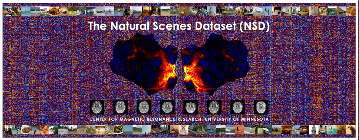
We will load from the Natural Scene Dataset. NSD is a large 7T fMRI dataset of 8 adults viewing more than 73,000 photos of natural scenes. We have taken a small subset of 90 images from NSD and have pre-extracted the fMRI data for V1 and Fusiform Face Area (FFA) from 8 subjects. Both of these areas are part of the visual cortex; V1 is known to respond to low-level visual features, while the FFA is famously responsive to high-level features, in particular faces.

Define constants#

Show image#

../../../_images/74eb65fc6b53ef4367d279cdc6d1d704402b402505d242a4d28ca00c7ab73396.png

Loading the images#

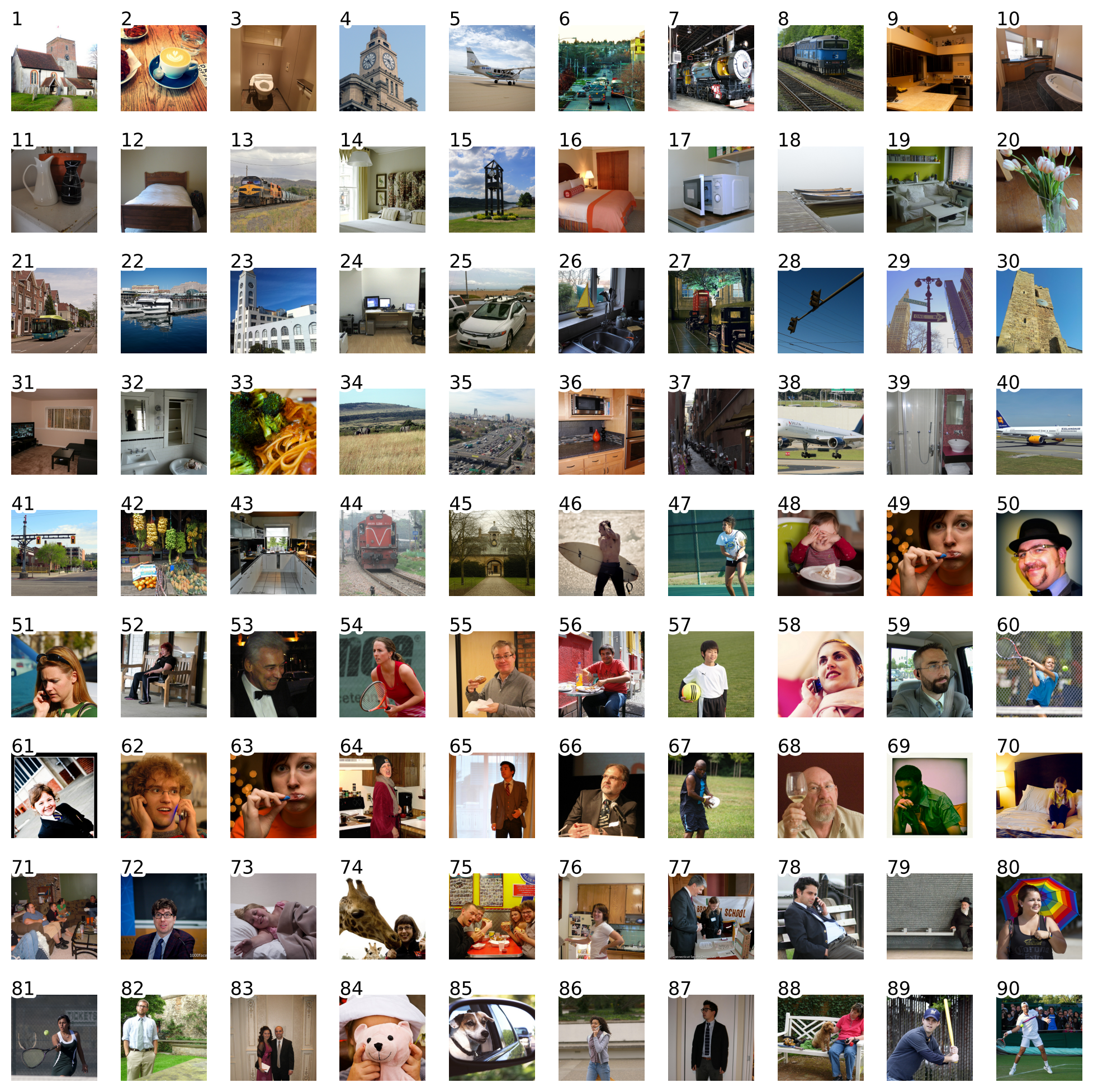
First, let’s load the 90 image files with the Pillow Image class.

Load the images and get image size#

(425, 425, 3)

Now, let’s take a look at these images. Notice that the first 45 images we selected have no faces, while the other 45 do have faces in them! So, we should expect to see a 2x2 block pattern in the Fusiform Face Area (FFA) representational dissimilarity matrices (RDMs).

Visualize images#

../../../_images/8d78dd9190ae4c234862197aab1ededc58ee1ca9b0ba7c0aa931a8403235d9de.png

Loading fMRI patterns from the NSD datset#

Let’s now load the fMRI patterns from the NSD dataset for these 90 images. We have pre-extracted the patterns, so we just need to load Numpy arrays from the .npy files.

Loading fMRI data#

(90, 2950)

Let’s now take a look at the pattern of responses for two non-face images and two face images.

def plot_fmri_pattern(subject, roi, image_idx, ax):
    pattern = fmri_patterns[subject][roi][image_idx]
    ax.plot(pattern)
    ax.set_title(f"Subject {subject}, ROI {roi}, Image {image_idx}")
    ax.set_xlabel("Voxel #")
    ax.set_ylabel("Activation")
    ax.set_xlim([200, 400])
    ax.set_ylim([-3, 3])


plt.figure(figsize=(8, 4))
ax = plt.gca()
subject = 1
roi = "FFA"

# non-face images
plot_fmri_pattern(subject, roi, 1, ax)
plot_fmri_pattern(subject, roi, 3, ax)

# face images
plot_fmri_pattern(subject, roi, 57, ax)
plot_fmri_pattern(subject, roi, 75, ax)

plt.legend(['non-face 1', 'non-face 2', 'face 1', 'face 2'])
plt.show()

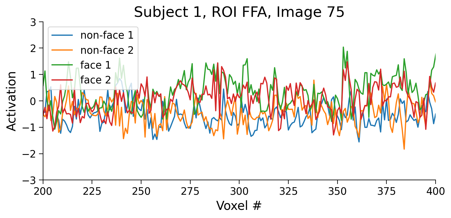
../../../_images/9a878f649508ff3b16d72d0ec4d47bb3002ba45f7e1dbea6cf7222ff5a41c46b.png

The activity is complex, but we clearly see several voxels (e.g., voxel 275) that have higher activation for faces than for non-faces. This is as expected for the face-selective FFA.

Submit your feedback#

Section 2: Get artificial neural network activations#

Estimated timing to here from start of tutorial: 15 minutes

Now that we have fMRI patterns, we want to explain this data using computational models.

In this tutorial, we will take our models to be layers of AlexNet.

Comparing LeNet architecture to AlexNet. Image from Dive Into Deep Learning book.

We load a version of AlexNet that is already pre-trained on ImageNet. This step may take a minute; feel free to read ahead.

Load AlexNet model pretrained on ImageNet#

To pass images through the model, we need to preprocess them to be in the same format as the images shown to the model during training.

For AlexNet, this includes resizing the images to 224x224 and normalizing their color channels to particular values. We also need to turn them into PyTorch tensors.

Preprocess NSD images as input to AlexNet#

torch.Size([90, 3, 224, 224])

Let’s inspect AlexNet architecture to select some of the layers as our models.

Inspect architecture#

Architecture of AlexNet:
AlexNet(
  (features): Sequential(
    (0): Conv2d(3, 64, kernel_size=(11, 11), stride=(4, 4), padding=(2, 2))
    (1): ReLU(inplace=True)
    (2): MaxPool2d(kernel_size=3, stride=2, padding=0, dilation=1, ceil_mode=False)
    (3): Conv2d(64, 192, kernel_size=(5, 5), stride=(1, 1), padding=(2, 2))
    (4): ReLU(inplace=True)
    (5): MaxPool2d(kernel_size=3, stride=2, padding=0, dilation=1, ceil_mode=False)
    (6): Conv2d(192, 384, kernel_size=(3, 3), stride=(1, 1), padding=(1, 1))
    (7): ReLU(inplace=True)
    (8): Conv2d(384, 256, kernel_size=(3, 3), stride=(1, 1), padding=(1, 1))
    (9): ReLU(inplace=True)
    (10): Conv2d(256, 256, kernel_size=(3, 3), stride=(1, 1), padding=(1, 1))
    (11): ReLU(inplace=True)
    (12): MaxPool2d(kernel_size=3, stride=2, padding=0, dilation=1, ceil_mode=False)
  )
  (avgpool): AdaptiveAvgPool2d(output_size=(6, 6))
  (classifier): Sequential(
    (0): Dropout(p=0.5, inplace=False)
    (1): Linear(in_features=9216, out_features=4096, bias=True)
    (2): ReLU(inplace=True)
    (3): Dropout(p=0.5, inplace=False)
    (4): Linear(in_features=4096, out_features=4096, bias=True)
    (5): ReLU(inplace=True)
    (6): Linear(in_features=4096, out_features=1000, bias=True)
  )
)

Graph node names (layers) in the forward pass:
['x', 'features.0', 'features.1', 'features.2', 'features.3', 'features.4', 'features.5', 'features.6', 'features.7', 'features.8', 'features.9', 'features.10', 'features.11', 'features.12', 'avgpool', 'flatten', 'classifier.0', 'classifier.1', 'classifier.2', 'classifier.3', 'classifier.4', 'classifier.5', 'classifier.6']

We extract activations from different layers of AlexNet processing the same images that were presented to people during the NSD task.

Make hooks in AlexNet to extract activations from different layers#

Extract activations from AlexNet#

(90, 46656)

Submit your feedback#

Section 3: Create representational dissimilarity matrices (RDMs)#

Estimated timing to here from start of tutorial: 20 minutes

Now that we have fMRI patterns and AlexNet activations, the first step in representation similarity analysis (RSA) is to compute the representational dissimilarity matrices (RDMs). RSA characterizes the representational geometry of the brain region of interest (ROI) by estimating the representational distance for each pair of experimental conditions (e.g., different images).

RDMs represent how dissimilar neural activity patterns or model activations are for each stimulus. In our case, these will be 90x90 image-by-image matrices representing how dissimilar fMRI patterns or AlexNet layer activations are for each image.

For instance, we expect that in FFA, there will be a large distance between the 45 face and 45 non-face images: we expect to see a 2x2 block pattern inside the RDM.

Creating RSA toolbox datasets#

First, let’s wrap our neural and model data in Dataset objects to use the RSA toolbox.

Create RSA datasets for each subject and ROI#

Create RSA datasets for AlexNet activations#

Computing the RDMs#

Let’s compute RDMs for fMRI patterns and AlexNet activations.

Compute rdms for each subject and ROI#

Coding Exercise 1: RDMs of AlexNet#

Use the RSA toolbox to compute the RDMs for the layers of AlexNet. It should be done in the very same way as RDMs for fMRI patterns above.

#################################################
## TODO for students: fill in the missing variables ##
# Fill out function and remove
raise NotImplementedError("Student exercise: fill in the missing variables")
#################################################

# Compute rdms for each layer of AlexNet
alexnet_rdms_dict = {}
for layer, dataset in alexnet_datasets.items():
    alexnet_rdms_dict[layer] = ...

Click for solution

Submit your feedback#

Visualizing human RDMs#

Here we use methods on the rsatoolbox RDM object to select a subset of the RDMs.

fmri_rdms = rsa.rdm.concat(fmri_rdms_list)
ffa_rdms = fmri_rdms.subset('roi', 'FFA')
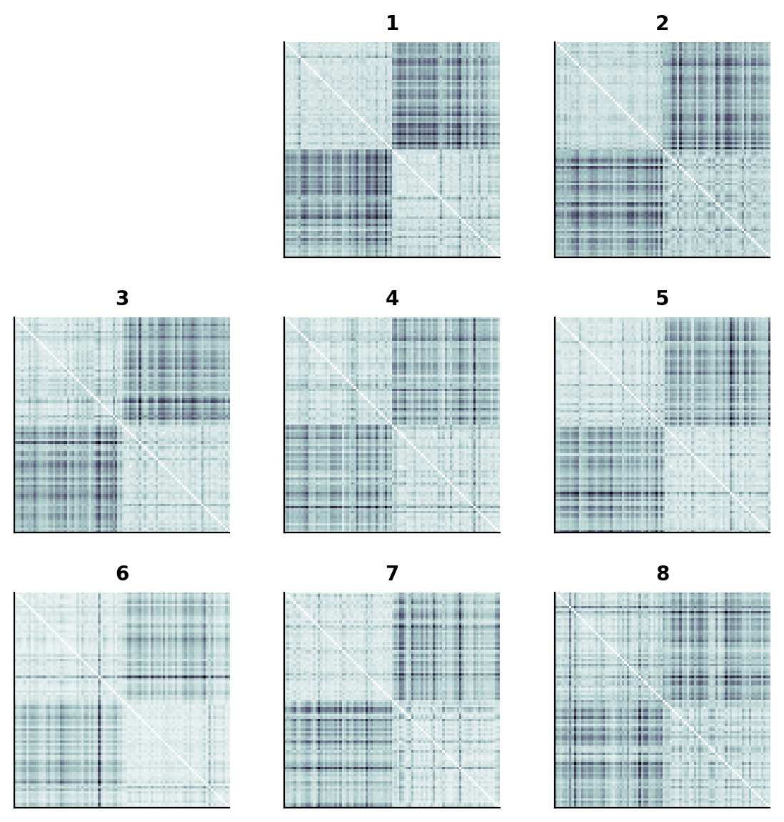
show_rdm_plotly(ffa_rdms, rdm_descriptor='subject')

As predicted above, we can see a 2x2 block-like pattern in the FFA fMRI pattern RDMs.

This is because we have 45 non-face images followed by 45 face images.

The lighter regions indicate larger representational distances.

# the same RDMs, using a different visualization method
fmri_rdms = rsa.rdm.concat(fmri_rdms_list)
fig = rsa.vis.rdm_plot.show_rdm(ffa_rdms, rdm_descriptor='subject')[0]

../../../_images/847c02eb74c165869cb5227457db0c8ed75d49af4e0a75cf180ecb8d0f88ae8d.png

Coding Exercise 2: Human RDMs#

Visualize the RDMs for the fMRI patterns from the V1 region.

fmri_rdms = rsa.rdm.concat(fmri_rdms_list)

#################################################
## TODO for students: fill in the missing variables ##
# Fill out function and remove
raise NotImplementedError("Student exercise: fill in the missing variables")
#################################################
v1_rdms = fmri_rdms.subset('roi', ...)
show_rdm_plotly(v1_rdms, rdm_descriptor='subject')

Click for solution

Submit your feedback#

Visualizing AlexNet RDMs#

Let’s look at RDMs for different layers of AlexNet.

alexnet_rdms = rsa.rdm.concat(alexnet_rdms_dict.values())
fig = rsa.vis.rdm_plot.show_rdm(alexnet_rdms, rdm_descriptor='layer')[0]

Each RDM contains the dissimilarities for each pair of activation patterns extracted by the different layers.

We see a similar pattern emerge, clustering face and non-face images in fully connected fc6, fc7, and fc8 layers.

AlexNet seems to represent faces differently than non-faces, at least to some extent.

# same RDMs, different visualization method
show_rdm_plotly(alexnet_rdms, rdm_descriptor='layer')

Submit your feedback#

Section 4: RSA. Model comparison and statistical inference#

Estimated timing to here from start of tutorial: 35 minutes

In the second step of RSA, each model is evaluated by the accuracy of its prediction of the data RDM. To this end, we will use the RDMs we computed for each model representation.

Each model’s prediction of the data RDM is evaluated using an RDM comparator. In this case, we will use the correlation coefficient.

First, let’s look at the performance of different Alexnet layers across all subjects.

Get the Model objects to use the rsa toolbox for model comparisons#

Visualize AlexNet performance#

In the plot, each data point represents the representational dissimilarity matrix (RDM) for an individual subject. The Y-axis indicates the correlation distance of the data RDMs to the RDM obtained from representations from each model layer. Each bar shows the mean correlation distance between data RDMs (across subjects) and one model layer. The observed variability reflects the extent to which our models (layers) accurately predict neural activity patterns across different individuals.

Our goal is to determine how these results might generalize to a new cohort of subjects and new sets of stimuli (assuming the new subjects and stimuli are sampled from the same respective populations). Since we cannot practically rerun the experiment countless times with fresh subjects and stimuli, we turn to computational simulations.

To achieve this, we will employ bootstrap resampling—a statistical technique that involves resampling our existing dataset with replacement to generate multiple simulated samples. This approach allows us to mimic the process of conducting the experiment anew with different subjects and/or different stimuli.

First, we’ll focus on generalization to new subjects. By bootstrapping the subject dataset for each simulated sample, we can compute the predictive accuracy of our models on the subjects’ RDMs. After running many simulations, we will accumulate a distribution of mean accuracy estimates that simulates the distribution of mean accuracies we might have obtained if we had actually repeated the experiment many times. This distribution will enable us to perform statistical inferences about our models’ generalizability to new subjects. Later, we will address the problem of generalizing to new stimuli as well.

Let’s simulate a new sample of subjects by bootstrap resampling using the RSA toolbox.

boot_rdms, idx = rsa.inference.bootstrap_sample_rdm(human_rdms, rdm_descriptor='subject')

Now, we plot the RDMs of the bootstrapped sample.

Each RDM is a subject (note that some subjects might be repeated and some might be missing in the bootstrapped sample).

Visualize RDMs#

As before, each RDM contains the pairwise dissimilarities between activation patterns in the specified brain region (in this case, FFA) for each of the subjects.

The first row shows the RDMs for each of the original 8 subjects. The second row shows 8 RDMs sampled from the set of 8 original RDMs with replacement. This is bootstrap resampling. It can be seen as a simulation of a “new” set of 8 subjects’ RDMs. Notice that in this new set not all subjects are represented and some others might appear more than once.

The idea is to see how the results for the model evaluations would change had our data come from this simulated sample of subjects.

Let’s see the model performance on different bootstrap resampled subject sets.

Visualize model evaluations#

If you run the cell above again, you will see the model performance for a new bootstrap sample of subjects.

Discussion#

Explore the results for a few simulated new cohorts: run the cell above a few times and see how to points (individual RDMs) and bars (means) change.

Hint: For different simulated sets of subjects, the mean correlation of their RDMs to the RDMs given by each layer may look quite different. For example, if a given subject’s RDM correlates very closely with layer conv4, and that subject is overrepresented in the bootstrap sample, the layer conv4 might yield a higher accuracy compared to the other layers.

Comparing representations statistically#

How can we know if these differences in model performance are statistically significant?

That is what the third and final step of RSA does: we conduct inferential comparisons between models based on their accuracy in predicting the representational dissimilarity matrices (RDMs).

We leverage the variability in the performance estimates observed in the bootstrapped samples to conduct statistical tests. These tests are designed to determine whether the differences in RDM prediction accuracy between models are statistically significant.

plot_model_comparison_trans(result)

The Y-axis, again, shows RDM prediction accuracy, as measured by the correlation between the data RDMs and the model RDMs. The error bars reflect the variability in this estimate across bootstrap samples over subjects). The gray bar indicates the noise ceiling, which is a measure of how well the best possible model (capturing the true data-generating process) could do, given the noise and intersubject variability in the data. The gray arrows indicate the models that don’t perform significantly better than the noise-ceiling. The white dots at the bottom of the bars indicate the models whose correlation distance to the data RDMs is significantly better than zero.

Details of the figure above#

Model comparisons are performed using a two-tailed t-test, FDR q < 0.01. Error bars indicate the standard error of the mean. One-sided comparisons of each model’s performance against 0 and against the lower-bound estimate of the noise ceiling are Bonferroni-corrected for the number of models.

Generalization to new images#

We have applied a method that enables us to infer how well the models might perform when predicting neural activity patterns for a new cohort of subjects. However, this approach has not yet considered the variability that would arise when replicating the experiment with a new sample of stimuli.

To make statistical inferences expected to generalize to new stimuli, we will once again use a bootstrapping procedure, focusing this time on the stimuli rather than the subjects.

To do this, we will first maintain the original cohort of subjects and apply bootstrapping to resample the stimulus set. That is, for each subject, we will sample a new RDM based on the RDM from that subject’s original activation patterns. The RDM will contain the pairwise dissimilarities between the response patterns to a set of stimuli sampled with replacement from the original set of stimuli.

Get the RDMs for a bootstrap sample of the images#

As before, rerunning the cell above will show you the RDMs for a new set of bootstrap-resampled stimuli each time.

Note that the block-like structure from before is generally preserved. This is because the stimuli are sorted so that the face stimuli are still adjacent to other face stimuli, and non-face stimuli are adjacent to other non-face stimuli. What changes are the specific stimuli used when computing the RDM. For each bootstrap resample, some stimuli might appear more than once, and some might be left out.

Let’s see the inferential model comparisons based on 1000 bootstraps of the image set.

result = rsa.inference.eval_bootstrap_pattern(models, human_rdms, theta=None, method='corr', N=1000,
                           pattern_descriptor='index', rdm_descriptor='index',
                           boot_noise_ceil=True)

plot_model_comparison_trans(result)

The Y-axis shows RDM prediction accuracy, as measured by the correlation distance between the data RDMs and the model RDMs. The error bars reflect the variability in this estimate across bootstrap samples (over stimuli). The gray bar indicates the noise ceiling, which is a measure of how well any model could do, given the noise in the data. The gray arrows indicate the models that don’t perform significantly better than the noise-ceiling. The white dots at the bottom of the bars indicate the models whose correlation distance to the data RDMs is significantly better than zero.

Details of the figure above#

Model comparisons: two-tailed t-test, FDR q < 0.01. Error bars indicate the standard error of the mean. One-sided comparisons of each model’s performance against 0 and against the lower-bound estimate of the noise ceiling are Bonferroni-corrected for the number of models.

Submit your feedback#

Section 5: Model Comparison Using Two-factor Bootstrap#

Estimated timing to here from start of tutorial: 45 minutes

For generalization across both the subject and stimulus populations, we can use a two-factor bootstrap method. For an in-depth discussion of this technique, refer to Schütt et al., 2023.

We can use the RSA toolbox to implement bootstrap resampling of subjects and stimuli simultaneously. It is important to note that a naive 2-factor bootstrap approach triple-counts the variance contributed by the measurement noise. For further understanding of this issue, see the explanation provided by Schütt et al. Fortunately, the RSA toolbox has an implementation that corrects this potential overestimation.

Let’s evaluate the performance of the models with simultaneous bootstrap resampling of the subjects and stimuli.

eval_result = rsa.inference.eval_dual_bootstrap(models, fmri_rdms.subset('roi', 'FFA'), method='corr')
print(eval_result)

plot_model_comparison_trans(eval_result)

In the plot above, the statistical comparison results take into account the variability in the data that comes from considering different sets of subjects and sets of stimuli.

Submit your feedback#

Summary#

Estimated timing of tutorial: 50 minutes

In this tutorial, we:

Reviewed the principles of RSA in the context of machine learning and computational neuroscience and applied it to the problem of comparing representations between fMRI patterns and neural network models for a vision task.
Explored the structure of AlexNet and extracted activations from the different layers of this neural network to a set of visual stimuli.
Evaluated how well the different layers of AlexNet could explain neural responses from humans to the same stimuli, by comparing the representations extracted from these layers (which we treated as different models) to the activity patterns derived from fMRI data.
Used frequentist statistical inference to compare the performance of the different model representations (i.e. layers).
Addressed two sources of model-performance estimation error that statistical inference must account for in addition to the error due to measurement noise: stimulus sampling and subject sampling, using the 2-factor bootstrap method.

Tutorial 3: Statistical inference on representational geometries

Contents

Tutorial 3: Statistical inference on representational geometries#

Tutorial Objectives#

Setup#

Install and import feedback gadget#

Import dependencies#

Figure settings#

Plotting functions#

Data retrieval#

Video 1: Tutorial Introduction#

Submit your feedback#

Section 1: Data Acquisition#

Define constants#

Show image#

Loading the images#

Load the images and get image size#

Visualize images#

Loading fMRI patterns from the NSD datset#

Loading fMRI data#

Submit your feedback#

Section 2: Get artificial neural network activations#

Load AlexNet model pretrained on ImageNet#

Preprocess NSD images as input to AlexNet#

Inspect architecture#

Make hooks in AlexNet to extract activations from different layers#

Extract activations from AlexNet#

Submit your feedback#

Section 3: Create representational dissimilarity matrices (RDMs)#

Creating RSA toolbox datasets#

Create RSA datasets for each subject and ROI#

Create RSA datasets for AlexNet activations#

Computing the RDMs#

Compute rdms for each subject and ROI#

Coding Exercise 1: RDMs of AlexNet#

Submit your feedback#

Visualizing human RDMs#

Coding Exercise 2: Human RDMs#

Submit your feedback#

Visualizing AlexNet RDMs#

Submit your feedback#

Section 4: RSA. Model comparison and statistical inference#

Get the Model objects to use the rsa toolbox for model comparisons#

Visualize AlexNet performance#

Visualize RDMs#

Visualize model evaluations#

Discussion#

Comparing representations statistically#

Details of the figure above#

Generalization to new images#

Get the RDMs for a bootstrap sample of the images#

Details of the figure above#

Submit your feedback#

Section 5: Model Comparison Using Two-factor Bootstrap#

Submit your feedback#

Summary#