

Tutorial 1: Sparsity and Sparse Coding
Week 1, Day 5: Microcircuits
By Neuromatch Academy
Content creators: Noga Mudrik, Xaq Pitkow
Content reviewers: Yizhou Chen, RyeongKyung Yoon, Ruiyi Zhang, Lily Chamakura, Hlib Solodzhuk, Patrick Mineault, Alex Murphy
Production editors: Konstantine Tsafatinos, Ella Batty, Spiros Chavlis, Samuele Bolotta, Hlib Solodzhuk, Alex Murphy
Tutorial Objectives
Estimated timing of tutorial: 1 hour 20 minutes
In this tutorial, we will discuss the notion of sparsity. In particular, we will:
Recognize various types of sparsity (population, lifetime, interaction).
Relate sparsity to inductive bias, interpretability, and efficiency.
Setup
Install and import feedback gadget
Source
# @title Install and import feedback gadget

!pip install vibecheck datatops --quiet

from vibecheck import DatatopsContentReviewContainer
def content_review(notebook_section: str):
    return DatatopsContentReviewContainer(
        "",  # No text prompt
        notebook_section,
        {
            "url": "https://pmyvdlilci.execute-api.us-east-1.amazonaws.com/klab",
            "name": "neuromatch_neuroai",
            "user_key": "wb2cxze8",
        },
    ).render()


feedback_prefix = "W1D5_T1"
Imports
Source
# @title Imports

#working with data
import numpy as np
import pandas as pd
from scipy.stats import kurtosis

#plotting
import matplotlib.pyplot as plt
import seaborn as sns
import logging
import matplotlib.patheffects as path_effects

#interactive display
import ipywidgets as widgets
from ipywidgets import interact, IntSlider
from tqdm.notebook import tqdm as tqdm

#modeling
from sklearn.datasets import make_sparse_coded_signal, make_regression
from sklearn.decomposition import DictionaryLearning, PCA
from sklearn.linear_model import OrthogonalMatchingPursuit
import tensorflow as tf

#utils
import os
import warnings
warnings.filterwarnings("ignore")
2026-07-07 03:48:00.764443: W tensorflow/stream_executor/platform/default/dso_loader.cc:64] Could not load dynamic library 'libcudart.so.11.0'; dlerror: libcudart.so.11.0: cannot open shared object file: No such file or directory; LD_LIBRARY_PATH: /opt/hostedtoolcache/Python/3.10.20/x64/lib
2026-07-07 03:48:00.764489: I tensorflow/stream_executor/cuda/cudart_stub.cc:29] Ignore above cudart dlerror if you do not have a GPU set up on your machine.
Figure settings
Source
# @title Figure settings

logging.getLogger('matplotlib.font_manager').disabled = True
sns.set_context('talk')

%matplotlib inline
%config InlineBackend.figure_format = 'retina' # perfrom high definition rendering for images and plots
plt.style.use("https://raw.githubusercontent.com/NeuromatchAcademy/course-content/main/nma.mplstyle")
Plotting functions
Source
# @title Plotting functions

def show_slice(slice_index):
    """
    Plot one slide of sequential data.

    Inputs:
    - slice_index (int): index of the slide to plot.
    """
    with plt.xkcd():
        plt.figure(figsize=(6, 6))
        plt.imshow(data[slice_index])
        ind = (66,133)
        plt.scatter([ind[1]], [ind[0]], facecolors='none', edgecolors='r', marker='s', s = 100, lw = 4)
        plt.axis('off')
        plt.show()

def remove_edges(ax, include_ticks = True, top = False, right = False, bottom = True, left = True):
    ax.spines['top'].set_visible(top)
    ax.spines['right'].set_visible(right)
    ax.spines['bottom'].set_visible(bottom)
    ax.spines['left'].set_visible(left)
    if not include_ticks:
        ax.get_xaxis().set_ticks([])
        ax.get_yaxis().set_ticks([])

def add_labels(ax, xlabel='X', ylabel='Y', zlabel='', title='', xlim = None, ylim = None, zlim = None,xticklabels = np.array([None]),
               yticklabels = np.array([None] ), xticks = [], yticks = [], legend = [],
               ylabel_params = {'fontsize':19},zlabel_params = {'fontsize':19}, xlabel_params = {'fontsize':19},
               title_params = {'fontsize':29}, format_xticks = 0, format_yticks = 0):
  """
  This function add labels, titles, limits, etc. to figures;
  Inputs:
      ax      = the subplot to edit
      xlabel  = xlabel
      ylabel  = ylabel
      zlabel  = zlabel (if the figure is 2d please define zlabel = None)
      etc.
  """
  if xlabel != '' and xlabel != None: ax.set_xlabel(xlabel, **xlabel_params)
  if ylabel != '' and ylabel != None:ax.set_ylabel(ylabel, **ylabel_params)
  if zlabel != '' and zlabel != None:ax.set_zlabel(zlabel,**zlabel_params)
  if title != '' and title != None: ax.set_title(title, **title_params)
  if xlim != None: ax.set_xlim(xlim)
  if ylim != None: ax.set_ylim(ylim)
  if zlim != None: ax.set_zlim(zlim)

  if (np.array(xticklabels) != None).any():
      if len(xticks) == 0: xticks = np.arange(len(xticklabels))
      ax.set_xticks(xticks);
      ax.set_xticklabels(xticklabels);
  if (np.array(yticklabels) != None).any():
      if len(yticks) == 0: yticks = np.arange(len(yticklabels)) +0.5
      ax.set_yticks(yticks);
      ax.set_yticklabels(yticklabels);
  if len(legend)       > 0:  ax.legend(legend)

def plot_signal(signal, title = "Pixel's activity over time", ylabel = '$pixel_t$'):
    """
    Plot the given signal over time.

    Inputs:
    - signal (np.array): given signal.
    - title (str, default = "Pixel's activity over time"): title to give to the plot.
    - ylabel (str, default = '$pixel_t$'): y-axis label.
    """
    with plt.xkcd():
        fig, ax = plt.subplots(1,1, figsize = (8,8), sharex = True)
        ax.plot(signal, lw = 2)
        ax.set_xlim(left = 0)
        ax.set_ylim(bottom = 0)
        add_labels(ax, xlabel = 'Time (Frames)',ylabel = ylabel, title = title)
        remove_edges(ax)
        plt.show()

def plot_relu_signal(signal, theta = 0):
    """
    Plot the given signal over time and its thresholded value with the given theta.

    Inputs:
    - signal (np.array): given signal.
    - theta (float, default = 0): threshold parameter.
    """
    with plt.xkcd():
        fig, ax = plt.subplots(1,1, figsize = (8,8), sharex = True)
        thres_x = ReLU(signal, theta)
        ax.plot(signal, lw = 2)
        ax.plot(thres_x, lw = 2)
        ax.set_xlim(left = 0)
        ax.legend(['Signal', '$ReLU_{%d}$(signal)'%theta], ncol = 2)
        add_labels(ax, xlabel = 'Time', ylabel = 'Signal')
        remove_edges(ax)
        plt.show()

def plot_relu_histogram(signal, theta = 0):
    """
    Plot histogram of the values in the signal before and after applying ReLU operation with the given threshold.

    Inputs:
    - signal (np.array): given signal.
    - theta (float, default = 0): threshold parameter.
    """
    with plt.xkcd():
        fig, axs = plt.subplots(1,2,figsize = (15,10), sharex = True, sharey = True)
        thres_x = ReLU(signal, theta)
        axs[0].hist(sig, bins = 100)
        axs[1].hist(thres_x, bins = 100)
        [remove_edges(ax) for ax in axs]
        [add_labels(ax, ylabel = 'Count', xlabel = 'Value') for ax in axs]
        [ax.set_title(title) for title, ax in zip(['Before Thresholding', 'After Thresholding'], axs)]
    plt.show()

def plot_relu_signals(signal, theta_values):
    """
    Plot the given signal over time and its thresholded value with the given theta values.

    Inputs:
    - signal (np.array): given signal.
    - theta_values (np.array): threshold parameter.
    """
    #define colormap
    with plt.xkcd():
        cmap_name = 'viridis'
        samples = np.linspace(0, 1, theta_values.shape[0])
        colors = plt.colormaps[cmap_name](samples)

        fig, ax = plt.subplots(1,1, figsize = (8,8), sharex = True)
        for counter, theta in enumerate(theta_values):
          ax.plot(ReLU(signal, theta), label = '$\\theta = %d$'%theta, color = colors[counter])
        ax.set_xlim(left = 0)
        ax.legend(ncol = 5)
        add_labels(ax, xlabel = 'Time', ylabel = '$ReLU_{\\theta}$(Signal)')
        remove_edges(ax)

def plot_images(images):
    """
    Plot given images.

    Inputs:
    - images (list): list of 2D np.arrays which represent images.
    """
    with plt.xkcd():
        fig, ax = plt.subplots(1, len(images), figsize = (15,8))
        if len(images) == 1:
            ax.imshow(images[0])
        else:
            for index, image in enumerate(images):
                ax[index].imshow(image)
    plt.show()

def plot_labeled_kurtosis(frame, frame_HT, labels = ['Frame', 'HT(frame)']):
    """
    Plot kurtosis value for the frame before and after applying hard threshold operation.

    Inputs:
    - frame (np.array): given image.
    - frame_HT (np.array): thresholded version of the given image.
    - labels (list): list of labels to apply for the igven data.
    """
    with plt.xkcd():
        fig, ax = plt.subplots()
        pd.DataFrame([kurtosis(frame.flatten()), kurtosis(frame_HT.flatten())],index = labels, columns = ['kurtosis']).plot.bar(ax = ax, alpha = 0.5, color = 'purple')
        remove_edges(ax)
    plt.show()

def plot_temporal_difference_histogram(signal, temporal_diff):
    """
    Plot histogram for the values of the given signal as well as for its temporal differenced version.

    Inputs:
    - signal (np.array): given signal.
    - temporal_diff (np.array): temporal differenced version of the signal.
    """
    with plt.xkcd():
        fig, axs = plt.subplots(1,2,figsize = (10,5), sharex = True, sharey = True)
        axs[0].hist(signal, bins = 100);
        axs[1].hist(temporal_diff, bins = 100);
        [remove_edges(ax) for ax in axs]
        [add_labels(ax, ylabel = 'Count', xlabel = 'Value') for ax in axs]
        [ax.set_title(title) for title, ax in zip(['Pixel \n Before Diff.', 'Frame \n After Diff.'], axs)]
        for line in axs[0].get_children():
            line.set_path_effects([path_effects.Normal()])
        for line in axs[1].get_children():
            line.set_path_effects([path_effects.Normal()])
        plt.show()

def plot_temp_diff_histogram(signal, taus, taus_list):
    """
    Plot the histogram for the given signal over time and its temporal differenced versions for different values of lag \tau.

    Inputs:
    - signal (np.array): given signal.
    - taus (np.array): array of tau values (lags).
    - taus_list (list): temporal differenced versions of the given signal.
    """
    #define colormap
    cmap_name = 'cool'
    samples = np.linspace(0, 1, taus.shape[0])
    colors = plt.colormaps[cmap_name](samples)

    with plt.xkcd():

        # histograms
        bin_edges = np.arange(0, 256, 5)  # Define bin edges from 0 to 255 with a step of 5

        # Compute histogram values using custom bin edges
        hist = [np.histogram(tau_list, bins=bin_edges)[0] for tau, tau_list in zip(taus, taus_list)]


        fig, ax = plt.subplots(figsize = (20,5))
        [ax.plot(bin_edges[:-1]*0.5 + bin_edges[1:]*0.5, np.vstack(hist)[j], marker = 'o', color = colors[j], label = '$\\tau = %d$'%taus[j]) for j in range(len(taus))]
        ax.legend(ncol = 2)
        remove_edges(ax)
        ax.set_xlim(left = 0, right = 100)
        add_labels(ax, xlabel = 'Value', ylabel = 'Count')
    plt.show()

def plot_temp_diff_separate_histograms(signal, lags, lags_list, tau = True):
    """
    Plot the histogram for the given signal over time and its temporal differenced versions for different values of lag \tau or windows.

    Inputs:
    - signal (np.array): given signal.
    - lags (np.array): array of lags (taus or windows).
    - lags_list (list): temporal differenced versions of the given signal.
    - tau (bool, default = True): which regime to use (tau or window).
    """
    with plt.xkcd():
        cmap_name = 'cool'
        samples = np.linspace(0, 1, lags.shape[0])
        colors = plt.colormaps[cmap_name](samples)

        fig, axs = plt.subplots(2, int(0.5*(2+lags.shape[0])),figsize = (15,10), sharex = True, sharey = False)
        axs = axs.flatten()
        axs[0].hist(signal, bins = 100, color = 'black');

        if tau:
            # histograms
            bin_edges = np.arange(0, 256, 5)  # Define bin edges from 0 to 255 with a step of 5

            # Compute histogram values using custom bin edges
            hist = [np.histogram(lag_list, bins=bin_edges)[0] for lag, lag_list in zip(lags, lags_list)]

            [axs[j+1].bar(bin_edges[:-1]*0.5 + bin_edges[1:]*0.5, np.abs( np.vstack(hist)[j]), color = colors[j]) for j in range(len(lags))]

        else:
            [axs[j+1].hist(np.abs(signal - diff_box_values_i), bins = 100, color = colors[j]) for j, diff_box_values_i in enumerate(lags_list)]

        [remove_edges(ax) for ax in axs]
        [add_labels(ax, ylabel = 'Count', xlabel = 'Value') for ax in axs]
        axs[0].set_title('Pixel \n Before Diff.');
        if tau:
            [ax.set_title( '$\\tau =$ %.2f'%lags[j]) for  j, ax in enumerate(axs[1:]) if j < lags.shape[0]]
        else:
            [ax.set_title( 'Window %d'%lags[j]) for  j, ax in enumerate(axs[1:]) if j < lags.shape[0]]

        for ax in axs:
            for line in ax.get_children():
                line.set_path_effects([path_effects.Normal()])
            for line in ax.get_children():
                line.set_path_effects([path_effects.Normal()])
    plt.show()

def plot_temp_diff_kurtosis(signal, lags, lags_list, tau = True):
    """
    Plot the kurtosis for the given signal over time and its temporal differenced versions for different values of lag \tau or windows.

    Inputs:
    - signal (np.array): given signal.
    - lags (np.array): array of lags (taus or windows).
    - lags_list (list): temporal differenced versions of the given signal.
    - tau (bool, default = True): which regime to use (tau or window).
    """
    with plt.xkcd():
        if tau:
            fig, ax = plt.subplots(figsize = (10,3))
            tauskur = [kurtosis(tau_i) for tau_i in lags_list]
            pd.DataFrame([kurtosis(signal)] + tauskur, index = ['Signal']+ ['$\\tau = {%d}$'%tau for tau in lags], columns = ['kurtosis']).plot.barh(ax = ax, alpha = 0.5, color = 'purple')
            remove_edges(ax)
        else:
            fig, ax = plt.subplots(figsize = (7,7))
            tauskur = [kurtosis(np.abs(signal - diff_box_values_i)) for diff_box_values_i in lags_list]
            pd.DataFrame([kurtosis(signal)] + tauskur, index = ['Signal']+ ['$window = {%d}$'%tau for tau in lags], columns = ['kurtosis']).plot.bar(ax = ax, alpha = 0.5, color = 'purple')
            remove_edges(ax)

def plot_diff_box(signal, filter, diff_box_signal):
    """
    Plot signal, the window function and the resulted convolution.

    Inputs:
    - signal (np.array): the given signal.
    - filter (int): size of the window function.
    - diff_box_signal (np.array): the resulted signal.
    """

    with plt.xkcd():
            fig, ax = plt.subplots(nrows=1, ncols=3, figsize=(15, 4))
            ax[0].plot(signal)
            ax[0].set_title('Signal')
            ax[1].plot(filter)
            ax[1].set_title('Filter Function')
            ax[2].plot(diff_box_signal)
            ax[2].set_title('diff_box Signal')
            plt.subplots_adjust(wspace=0.3)
            [ax_i.set_xlabel('Time') for ax_i in ax]
    plt.show()

def plot_diff_with_diff_box(signal, windows, diff_box_values):
    """
    Plot difference between given signal and diff_box ones for different windows.

    Inputs:
    - signal (np.array): given signal.
    - windows (np.array): list of window sizes.
    - diff_box_values (list): list for diff_box versions of the signal.
    """
    with plt.xkcd():
        cmap_name = 'cool'
        samples = np.linspace(0, 1, windows.shape[0])
        colors = plt.colormaps[cmap_name](samples)

        fig, ax = plt.subplots(figsize = (15,10))
        ax.plot(signal, label = "Signal")
        [ax.plot(signal - diff_box_values_i, color = colors[j], label = 'window = %d'%windows[j]) for j, diff_box_values_i in enumerate(diff_box_values)]
        ax.legend(ncol = 4)
        remove_edges(ax)
        ax.set_xlim(left = 0, right = 100)
        add_labels(ax, xlabel = 'Time (frame)', ylabel = '$\Delta(pixel)$')
    plt.show()

def plot_spatial_diff(frame, diff_x,  diff_y):
    """
    Plot spatial differentiation of the given image with lag one.

    Inputs:
    - frame (np.array): given 2D signal (image).
    - diff_x (np.array): spatial difference along x-axis.
    - diff_y (np.array): spatial difference along y-axis.
    """

    with plt.xkcd():
        fig, axs = plt.subplots(1,3, figsize = (15,10))
        diff_x_norm = (diff_x - np.percentile(diff_x, 10))/(np.percentile(diff_x, 90) - np.percentile(diff_x, 10))
        diff_x_norm = diff_x_norm*255
        diff_x_norm[diff_x_norm > 255] = 255
        diff_x_norm[diff_x_norm < 0] = 0
        axs[0].imshow(diff_x_norm.astype(np.uint8))
        diff_y_norm = (diff_y - np.percentile(diff_y, 10))/(np.percentile(diff_y, 90) - np.percentile(diff_y, 10))
        diff_y_norm = diff_y_norm*255
        diff_y_norm[diff_y_norm > 255] = 255
        diff_y_norm[diff_y_norm < 0] = 0
        axs[1].imshow(diff_y_norm.astype(np.uint8))
        axs[2].imshow(frame)
        [ax.set_xticks([]) for ax in axs]
        [ax.set_yticks([]) for ax in axs]
        [ax.set_title(title, fontsize = 40) for title, ax in zip(['$\Delta x$', '$\Delta y$', 'Original'], axs)];

def plot_spatial_diff_histogram(taus, taus_list_x, taus_list_y):
    """
    Plot histograms for each of the spatial differenced version of the signal.
    """

    with plt.xkcd():
        cmap_name = 'cool'
        samples = np.linspace(0, 1, taus.shape[0])
        colors = plt.colormaps[cmap_name](samples)

        bin_edges = np.arange(0, 256, 5)  # Define bin edges from 0 to 255 with a step of 5

        hist_x = [np.histogram(tau_list.flatten() ,  bins=bin_edges)[0] for tau, tau_list in zip(taus, taus_list_x )]
        hist_y = [np.histogram(tau_list.flatten(),  bins=bin_edges)[0] for tau, tau_list in zip(taus, taus_list_y)]

        fig, axs = plt.subplots(2,1,figsize = (15,9))
        ax = axs[0]
        [ax.plot(bin_edges[:-1]*0.5 + bin_edges[1:]*0.5, np.vstack(hist_x)[j], marker = 'o', color = colors[j], label = '$\\tau = %d$'%taus[j]) for j in range(len(taus))]
        ax.set_yscale('log')
        ax.legend(ncol = 2)
        remove_edges(ax)
        ax.set_xlim(left = 0, right = 100)
        add_labels(ax, xlabel = '$\\tau_x$', ylabel = 'Count', title = 'Diff. in $x$')

        ax = axs[1]
        [ax.plot(bin_edges[:-1]*0.5 + bin_edges[1:]*0.5, np.vstack(hist_y)[j], marker = 'o', color = colors[j], label = '$\\tau = %d$'%taus[j]) for j in range(len(taus))]
        ax.set_yscale('log')
        ax.legend(ncol = 2)
        remove_edges(ax)
        ax.set_xlim(left = 0, right = 100)
        add_labels(ax, xlabel = '$\\tau_y$', ylabel = 'Count', title = 'Diff. in $y$')

        fig.tight_layout()
    plt.show()

def plot_spatial_kurtosis(frame, diff_x, diff_y):
    """
    Plot kurtosis for the signal and its spatial differenced version.
    """
    with plt.xkcd():
        fig, ax = plt.subplots()
        pd.DataFrame([kurtosis(frame.flatten()), kurtosis(diff_x.flatten()), kurtosis(diff_y.flatten())],index = ['Signal', 'Diff $x$', 'Diff $y$'], columns = ['kurtosis']).plot.barh(ax = ax, alpha = 0.5, color = 'purple')
        remove_edges(ax)
    plt.show()

def plot_spatial_histogram(frame, diff_x, diff_y):
    """
    Plot histogram for values in frame and differenced versions.
    """
    with plt.xkcd():
        fig, axs = plt.subplots(1,3,figsize = (15,10), sharex = True, sharey = True)
        axs[0].hist(np.abs(frame.flatten()), bins = 100);
        axs[1].hist(np.abs(diff_x.flatten()), bins = 100);
        axs[2].hist(np.abs(diff_y.flatten()), bins = 100);
        [remove_edges(ax) for ax in axs]
        [add_labels(ax, ylabel = 'Count', xlabel = 'Value') for ax in axs]
        [ax.set_title(title) for title, ax in zip(['Frame \n Before Diff.', 'Frame \n After Diff. x', 'Frame \n After Diff. y'], axs)]

def visualize_images_diff_box(frame, diff_box_values_x, diff_box_values_y, num_winds):
    """
    Plot images with diff_box difference method.
    """
    with plt.xkcd():
        cmap_name = 'cool'
        samples = np.linspace(0, 1, num_winds)
        colors = plt.colormaps[cmap_name](samples)
        fig, axs = plt.subplots( 2, int(0.5*(2+ len(diff_box_values_x))),  figsize = (15,15))
        axs = axs.flatten()
        axs[0].imshow(frame)
        [axs[j+1].imshow(normalize(frame - diff_box_values_i)) for j, diff_box_values_i in enumerate(diff_box_values_x)]
        remove_edges(axs[-1], left = False, bottom = False, include_ticks=  False)
        fig.suptitle('x diff')

        fig, axs = plt.subplots( 2, int(0.5*(2+ len(diff_box_values_x))),  figsize = (15,15))
        axs = axs.flatten()
        axs[0].imshow(frame)
        [axs[j+1].imshow(normalize(frame.T - diff_box_values_i).T) for j, diff_box_values_i in enumerate(diff_box_values_y)]
        remove_edges(axs[-1], left = False, bottom = False, include_ticks=  False)
        fig.suptitle('y diff')

def create_legend(dict_legend, size = 30, save_formats = ['.png','.svg'],
                      save_addi = 'legend' , dict_legend_marker = {},
                      marker = '.', style = 'plot', s = 500, plot_params = {'lw':5},
                      params_leg = {}):
    fig, ax = plt.subplots(figsize = (5,5))
    if style == 'plot':
        [ax.plot([],[],
                     c = dict_legend[area], label = area, marker = dict_legend_marker.get(area), **plot_params) for area in dict_legend]
    else:
        if len(dict_legend_marker) == 0:
            [ax.scatter([],[], s=s,c = dict_legend.get(area), label = area, marker = marker, **plot_params) for area in dict_legend]
        else:
            [ax.scatter([],[], s=s,c = dict_legend[area], label = area, marker = dict_legend_marker.get(area), **plot_params) for area in dict_legend]
    ax.legend(prop = {'size':size},**params_leg)
    remove_edges(ax, left = False, bottom = False, include_ticks = False)

def ReLU_implemented(x, theta = 0):
    """
    Calculates ReLU function for the given level of theta (implemented version of first exercise).

    Inputs:
    - x (np.ndarray): input data.
    - theta (float, default = 0): threshold parameter.

    Outputs:
    - thres_x (np.ndarray): filtered values.
    """

    thres_x = np.maximum(x - theta, 0)

    return thres_x

def plot_kurtosis(theta_value):
    """
    Plot kurtosis value for the signal before and after applying ReLU operation with the given threshold value.

    Inputs:
    - theta_value (int):  threshold parameter value.
    """
    with plt.xkcd():
        fig, ax = plt.subplots()
        relu = kurtosis(ReLU_implemented(sig, theta_value))
        pd.DataFrame([kurtosis(sig)] + [relu], index = ['Signal']+ ['$ReLU_{%d}$(signal)'%theta_value], columns = ['kurtosis']).plot.bar(ax = ax, alpha = 0.5, color = 'purple')
        remove_edges(ax)
        plt.show()
Data retrieval
Source
# @title Data retrieval

import os
import requests
import hashlib

# Variables for file and download URL
fnames = ["frame1.npy", "sig.npy", "reweight_digits.npy", "model.npy", "video_array.npy"] # The names of the files to be downloaded
urls = ["https://osf.io/n652y/download", "https://osf.io/c9qxk/download", "https://osf.io/ry5am/download", "https://osf.io/uebw5/download", "https://osf.io/t9g2m/download"] # URLs from where the files will be downloaded
expected_md5s = ["6ce619172367742dd148cc5830df908c", "f3618e05e39f6df5997f78ea668f2568", "1f2f3a5d08e13ed2ec3222dca1e85b60", "ae20e6321836783777c132149493ec70", "bbd1d73eeb7f5c81768771ceb85c849e"] # MD5 hashes for verifying files integrity

for fname, url, expected_md5 in zip(fnames, urls, expected_md5s):
    if not os.path.isfile(fname):
        try:
            # Attempt to download the file
            r = requests.get(url) # Make a GET request to the specified URL
        except requests.ConnectionError:
            # Handle connection errors during the download
            print("!!! Failed to download data !!!")
        else:
            # No connection errors, proceed to check the response
            if r.status_code != requests.codes.ok:
                # Check if the HTTP response status code indicates a successful download
                print("!!! Failed to download data !!!")
            elif hashlib.md5(r.content).hexdigest() != expected_md5:
                # Verify the integrity of the downloaded file using MD5 checksum
                print("!!! Data download appears corrupted !!!")
            else:
                # If download is successful and data is not corrupted, save the file
                with open(fname, "wb") as fid:
                    fid.write(r.content) # Write the downloaded content to a file
Helper functions
Source
# @title Helper functions

def normalize(mat):
    """
    Normalize input matrix from 0 to 255 values (in RGB range).

    Inputs:
    - mat (np.ndarray): data to normalize.

    Outpus:
    - (np.ndarray): normalized data.
    """
    mat_norm = (mat - np.percentile(mat, 10))/(np.percentile(mat, 90) - np.percentile(mat, 10))
    mat_norm = mat_norm*255
    mat_norm[mat_norm > 255] = 255
    mat_norm[mat_norm < 0] = 0
    return mat_norm

def lists2list(xss):
    """
    Flatten a list of lists into a single list.

    Inputs:
    - xss (list): list of lists. The list of lists to be flattened.

    Outputs:
    - (list): The flattened list.
    """
    return [x for xs in xss for x in xs]

# exercise solutions for correct plots

def ReLU(x, theta = 0):
    """
    Calculates ReLU function for the given level of theta.

    Inputs:
    - x (np.ndarray): input data.
    - theta (float, default = 0): threshold parameter.

    Outputs:
    - thres_x (np.ndarray): filtered values.
    """

    thres_x = np.maximum(x - theta, 0)

    return thres_x

sig = np.load('sig.npy')
temporal_diff = np.abs(np.diff(sig))

num_taus = 10
taus = np.linspace(1, 91, num_taus).astype(int)
taus_list = [np.abs(sig[tau:] - sig[:-tau]) for tau in taus]

T_ar = np.arange(len(sig))

freqs = np.linspace(0.001, 1, 100)
set_sigs = [np.sin(T_ar*f) for f in freqs]

reg = OrthogonalMatchingPursuit(fit_intercept = True, n_nonzero_coefs = 10).fit(np.vstack(set_sigs).T, sig)
Section 1: Introduction to sparsity
Video 1: Introduction to sparsity
Sparsity in Neuroscience and Artificial Intelligence
Sparse means rare or thinly spread out.
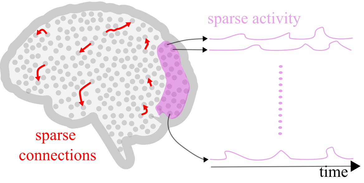
Neuroscience and AI both use notions of sparsity to describe efficient representations of the world. The concept of sparsity is usually applied to two things: sparse activity and sparse connections.
Sparse activity means that only a small number of neurons or units are active at any given time. Computationally, this helps reduce energy consumption and focuses computational efforts on the most salient features of the data. In modeling the world, it reflects how natural scenes usually contain a small number out of all possible objects or features.
Sparse connections refers to the selective interaction between neurons or nodes, for example, through a graph that is far from fully connected. Computationally, this can focus processing power where it is most needed. In modeling the world, it reflects that many represented objects or features properties directly relate only to a few others.
In the brain, we see sparsity of both types, and researchers have made many theories about its benefits. In AI, regularization often imposes sparsity, providing a variety of performance and generalization benefits.
This tutorial will explore a few of these benefits. First, we will calculate how various simple computations affect sparsity, and then we will examine how sparsity can affect inferences.
How can we quantify sparsity?
pseudo-norm -- the count of non-zero values: where is an indicator function equal to 1 if and only if the argument is true. This is more difficult to work with than other proxy measures that are convex or differentiable.
norm -- the sum of the absolute values:
Kurtosis -- a fourth-order measure that quantifies the “tails” of the distribution: . Higher kurtosis indicates both longer tails and smaller values and, thus, greater sparsity.
Cardinality -- in this context, refers to the number of active (non-zero) features in a model, which determines its sparsity and affects its ability to capture and express complex data patterns.
Section 2: Computing and altering sparsity
Estimated timing to here from start of tutorial: 10 minutes.
Under what scenarios do we encounter sparsity in real life? In this first section, we will explore various contexts and methods through which natural sparsity manifests in real-world signals. We will focus on the effects of nonlinearity and temporal derivatives.
Section 2.1: Sparsity via nonlinearity
Video 2: Natural sparsity
Coding Exercise 2.1: Sparsity as the result of thresholding
In this exercise, we will understand how a nonlinearity can increase sparsity.
For the first exercise, we will analyze a video of a bird in San Francisco to extract temporal sparsity. You can navigate through the video using the slider provided below.
Specifically, to explore temporal sparsity (i.e., sparsity across time, also called lifetime sparsity), we will focus on the activity of a particular pixel, the one marked in red, across various frames.
Execute the cell to see the interactive widget!
Source
# @title Execute the cell to see the interactive widget!

data = np.load('video_array.npy')
slider = IntSlider(min=0, max=data.shape[0] - 1, step=1, value=0, description= 'Time Point')
interact(show_slice, slice_index=slider)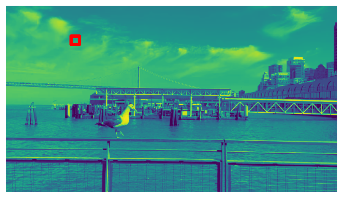
<function __main__.show_slice(slice_index)>Now, let’s look at the marked pixel’s activity over time and visualize it.
Plot of change in pixel’s value over time
Source
# @title Plot of change in pixel's value over time

sig = np.load('sig.npy')
plot_signal(sig)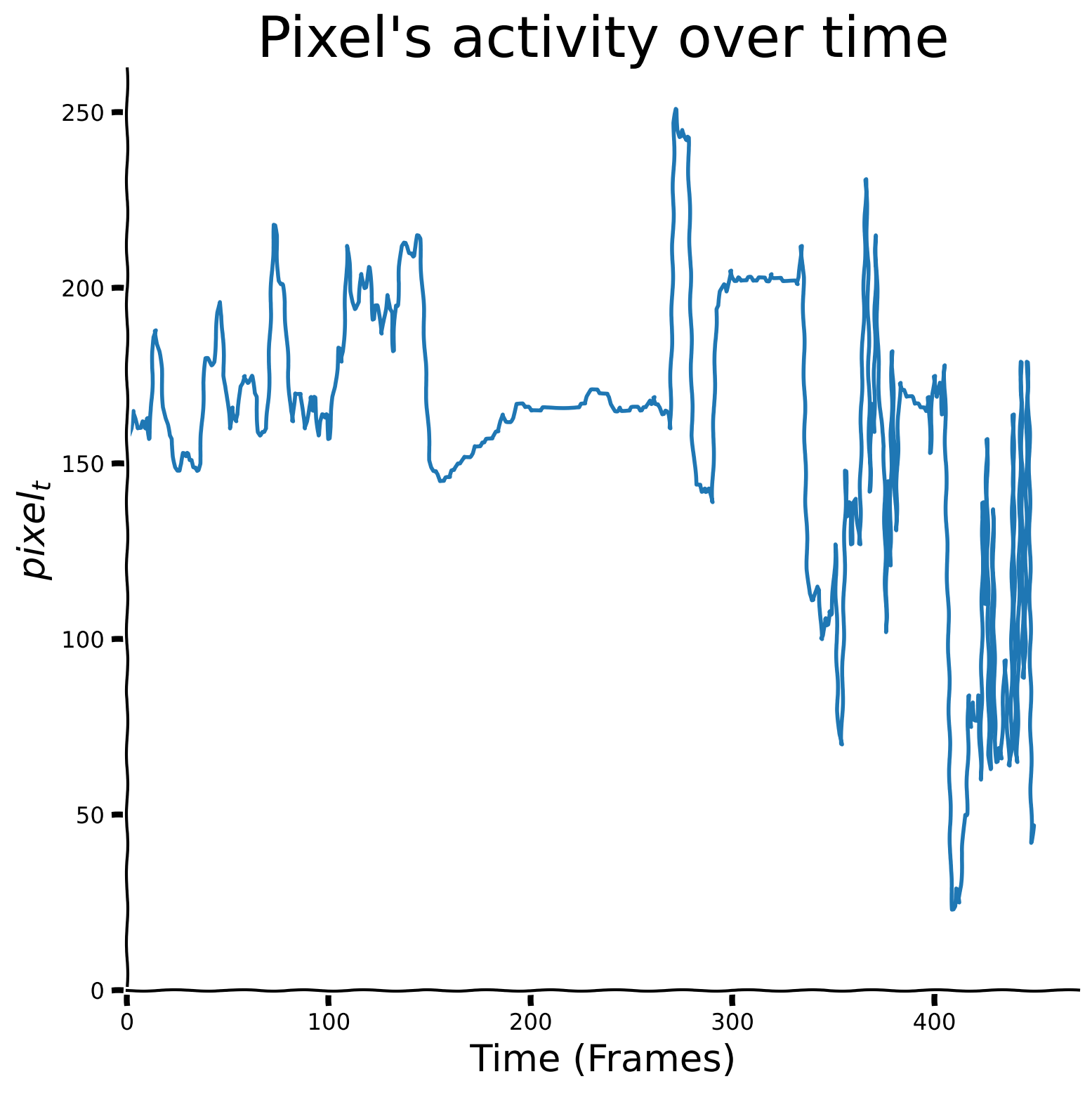
Write a function called “ReLU” that receives 2 inputs:
: a 1d numpy array of floats.
: a scalar threshold.
The function should return a numpy array called thres_x such that for each element :
Apply the ReLU function to the signal “sig” with a threshold of .
###################################################################
## Fill out the following then remove
raise NotImplementedError("Student exercise: complete `thres_x` array calculation as defined.")
###################################################################

def ReLU(x, theta = 0):
    """
    Calculates ReLU function for the given level of theta.

    Inputs:
    - x (np.ndarray): input data.
    - theta (float, default = 0): threshold parameter.

    Outputs:
    - thres_x (np.ndarray): filtered values.
    """

    thres_x = ...

    return thres_x
---------------------------------------------------------------------------
NotImplementedError Traceback (most recent call last)
Cell In[9], line 3
1 ###################################################################
2 ## Fill out the following then remove
----> 3 raise NotImplementedError("Student exercise: complete `thres_x` array calculation as defined.")
4 ###################################################################
6 def ReLU(x, theta = 0):
NotImplementedError: Student exercise: complete `thres_x` array calculation as defined.Plot your results
Source
# @title Plot your results

plot_relu_signal(sig, theta = 150)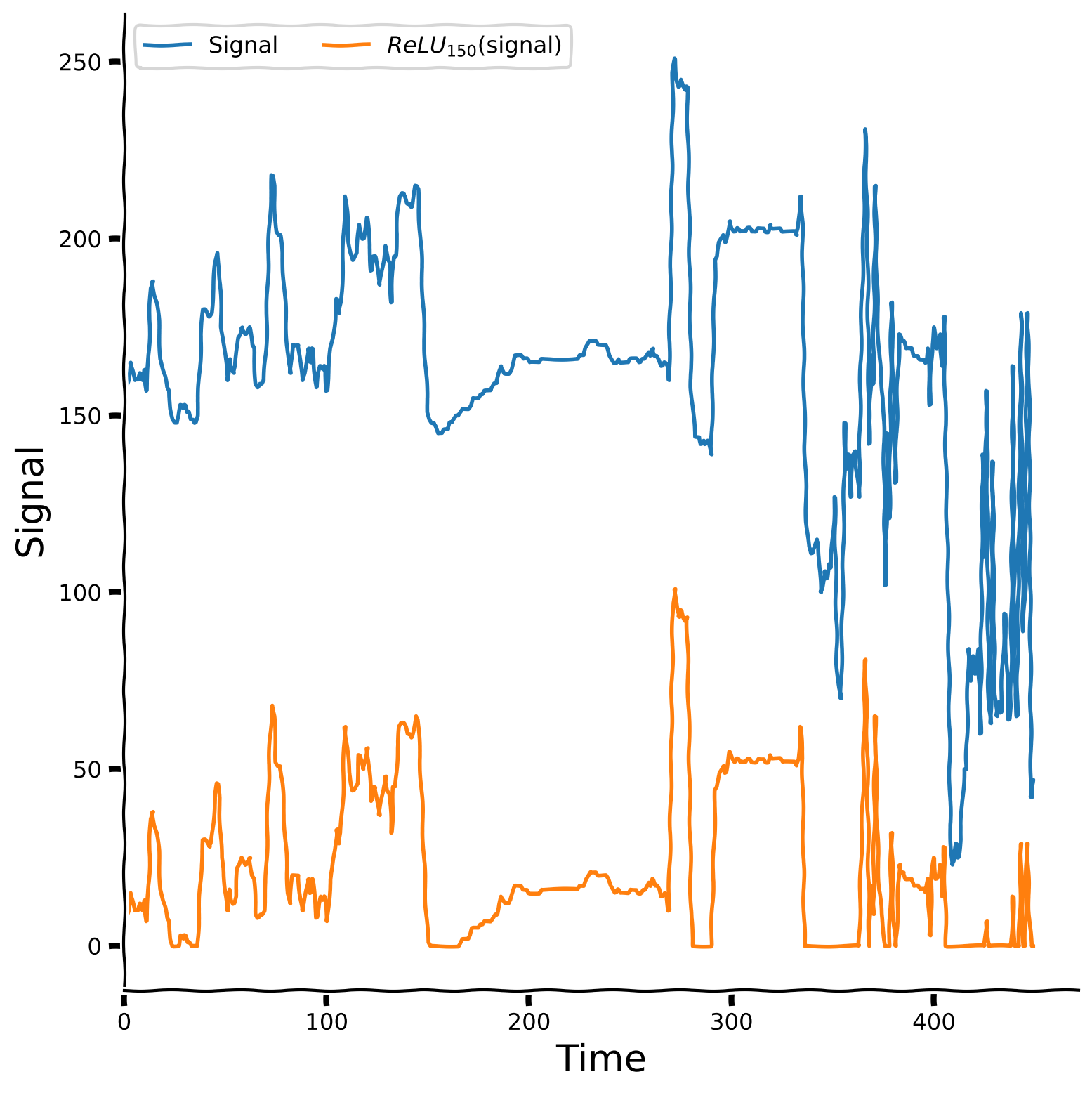
Let us also take a look at the aggregated plot, which takes threshold parameter values from 0 to 240 with step 20 and plots the ReLU version of the signal for each of them.
Threshold value impact on ReLU version of the signal
Source
# @title Threshold value impact on ReLU version of the signal

theta_values = np.arange(0, 240, 20)
plot_relu_signals(sig ,theta_values)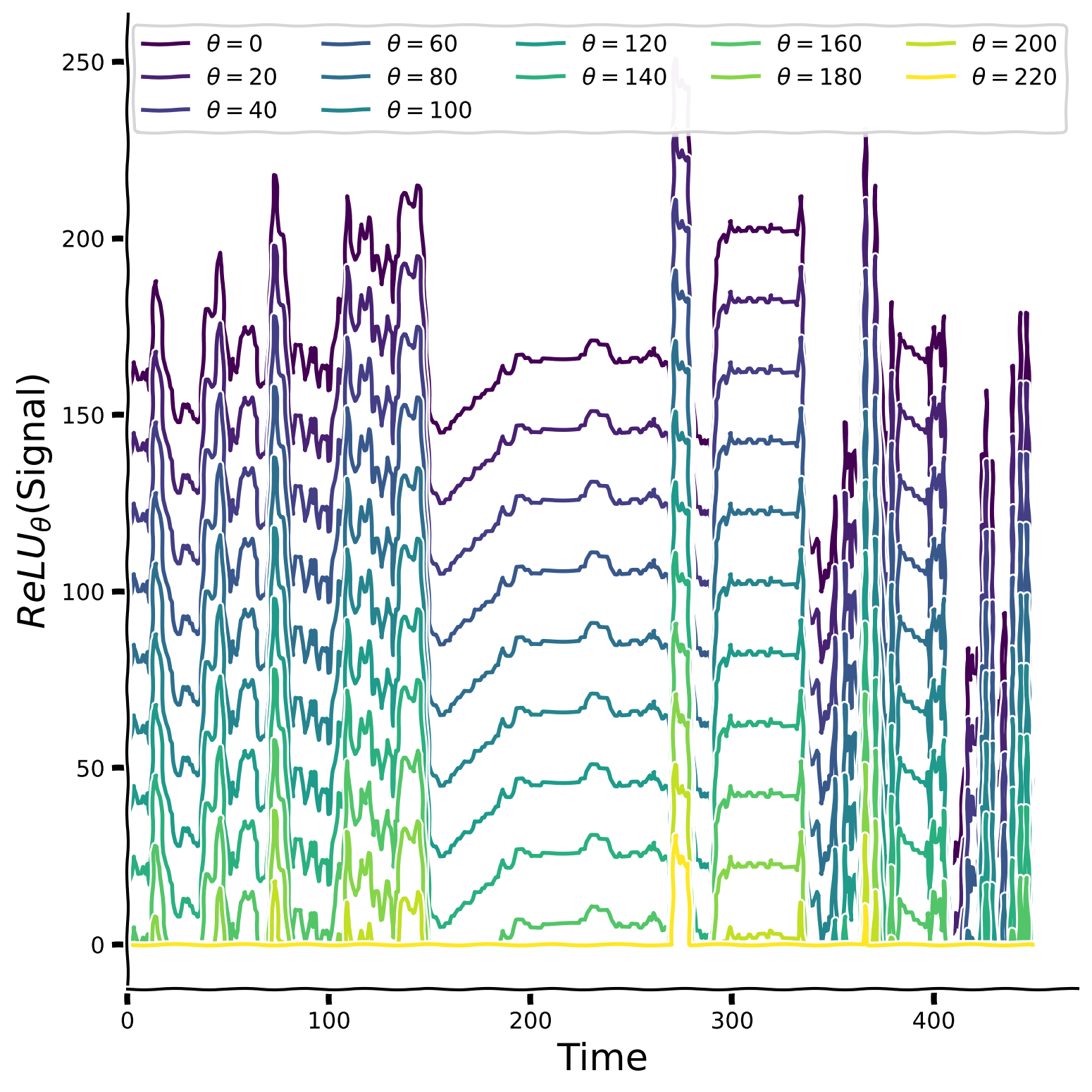
Finally, let’s calculate the kurtosis value to estimate the signal’s sparsity compared to its version passed through the ReLU function.
Try to gradually increase the threshold parameter () from 0 to 240 in intervals of 20 and plot the result for each value. How does the threshold affect the sparsity?
Kurtosis value comparison
Source
# @title Kurtosis value comparison

slider = IntSlider(min=0, max=240, step=20, value=0, description='Threshold')
interact(plot_kurtosis, theta_value = slider)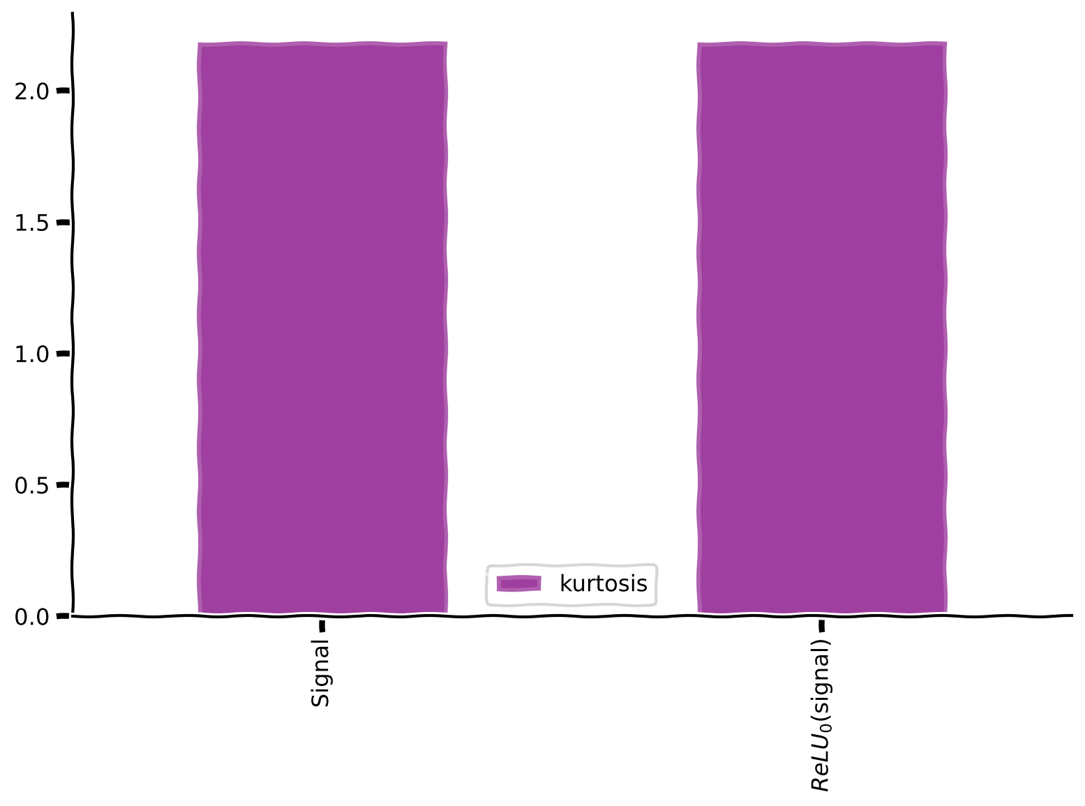
<function __main__.plot_kurtosis(theta_value)>Kurtosis value behaviour
Section 2.2: Sparsity from temporal differentiation
Estimated timing to here from start of tutorial: 20 minutes.
In this section, you will increase temporal sparsity in a natural 1D time series by temporal differencing. Changes in the world are sparse and thus tend to be especially informative, so computations highlighting those changes can be beneficial.
This could be implemented by feedforward inhibition in a neural circuit.
Video 3: Temporal differentiation
Coding Exercise 2.2: Temporal differencing signal
Denote the pixel value at time by . Mathematically, we define the (absolute) temporal differences as
In code, define these absolute temporal differences to compute temporal_diff by applying np.diff on the signal sig and then applying np.abs to get absolute values. The NumPy function np.diff takes in the signal as well as an additional parameter n which compares the value of element i with i-n (the default value is n=1). As a reminder, if not specified, then the default hyperparameter value is used.
###################################################################
## Fill out the following then remove
raise NotImplementedError("Student exercise: complete temporal differentiation.")
###################################################################
temporal_diff = ...
---------------------------------------------------------------------------
NotImplementedError Traceback (most recent call last)
Cell In[13], line 3
1 ###################################################################
2 ## Fill out the following then remove
----> 3 raise NotImplementedError("Student exercise: complete temporal differentiation.")
4 ###################################################################
5 temporal_diff = ...
NotImplementedError: Student exercise: complete temporal differentiation.Observe the result
Source
# @title Observe the result
plot_signal(temporal_diff, title = "", ylabel = "$| pixel_t - pixel_{t-1} | $")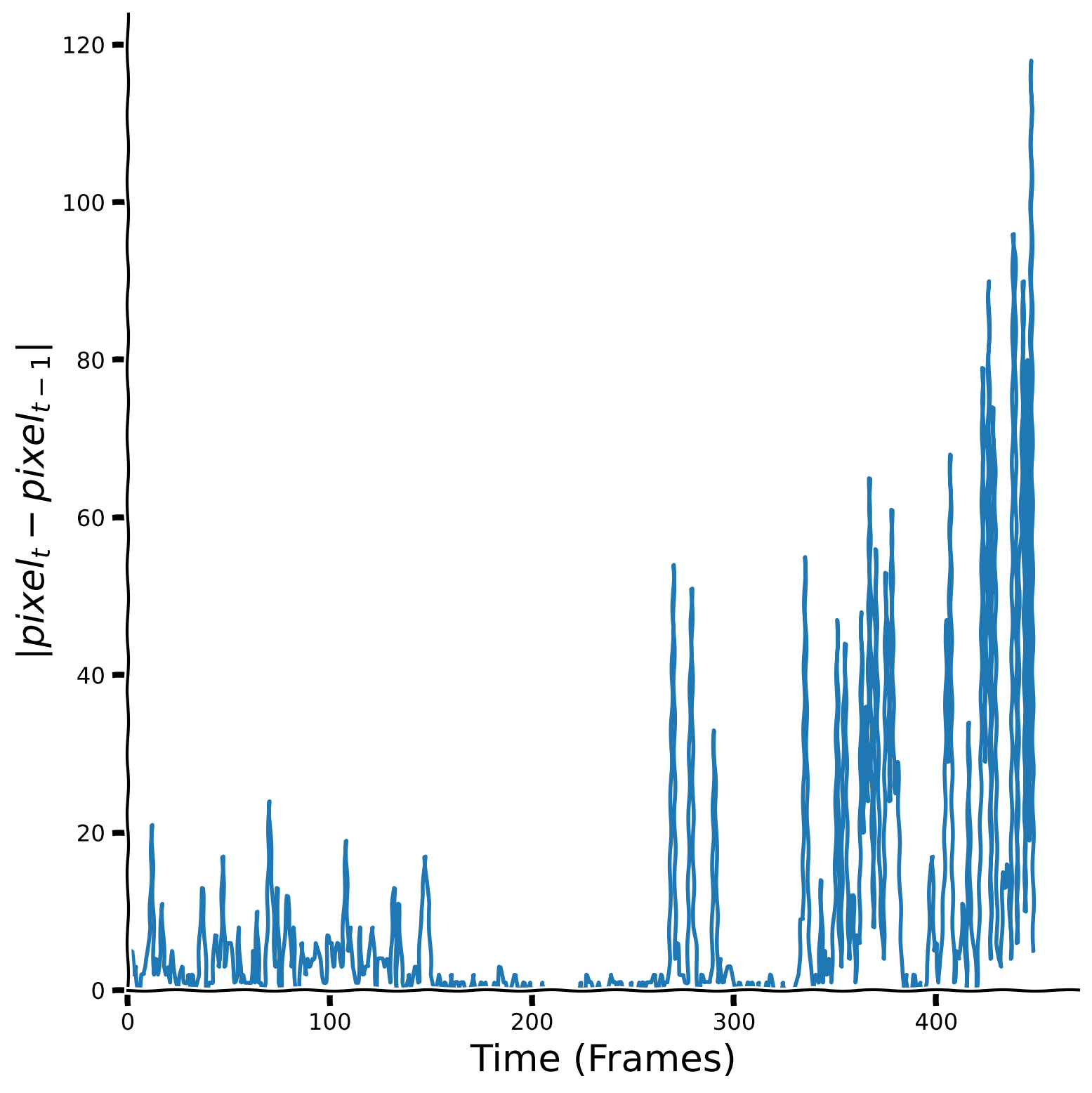
Let’s take a look at the histogram of the temporal difference values as well as kurtosis values.
Histograms for the signal and its temporal differences
Source
# @title Histograms for the signal and its temporal differences
plot_temporal_difference_histogram(sig, temporal_diff)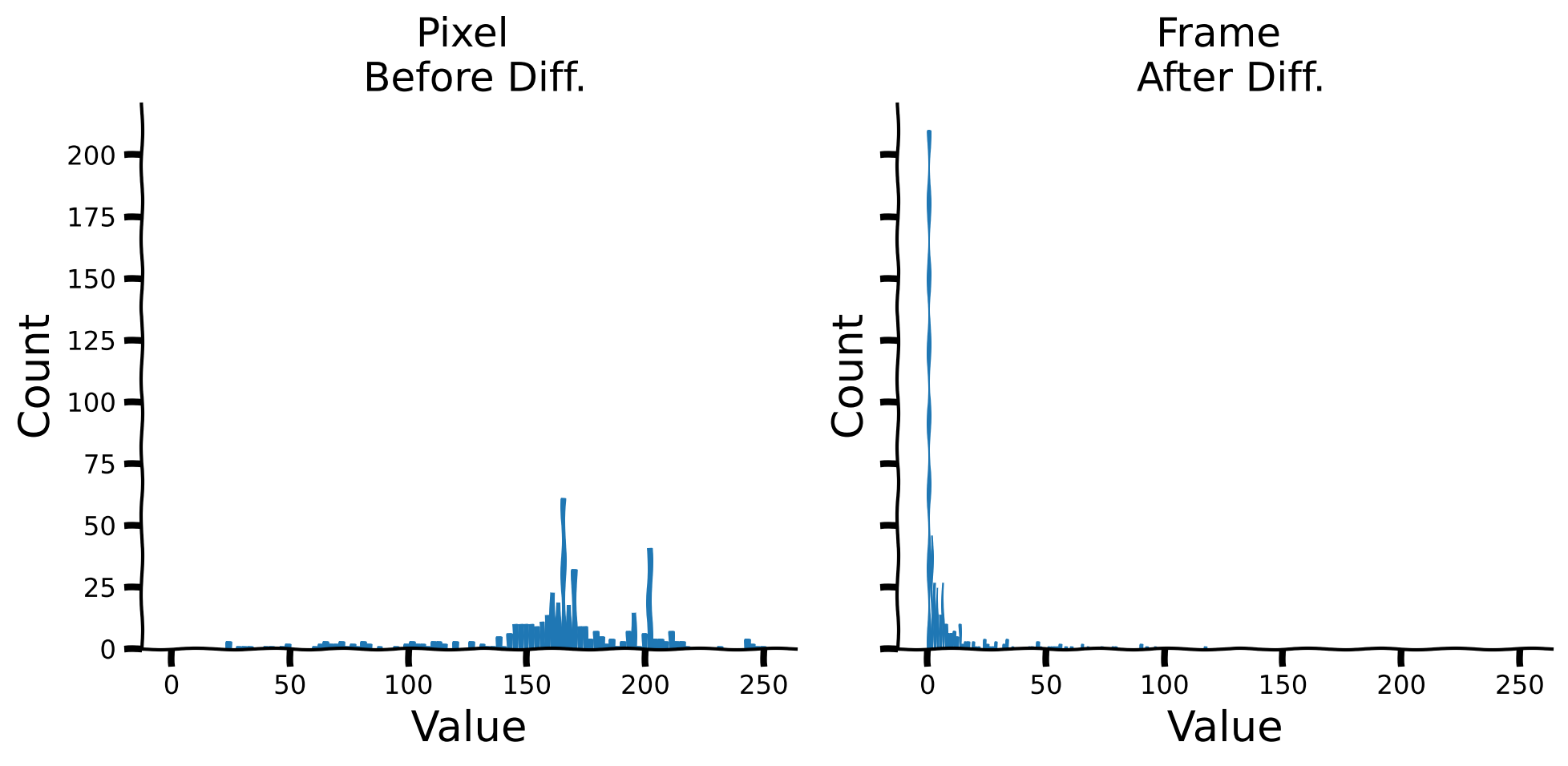
Kurtosis values for the signal and its temporal differences
Source
# @title Kurtosis values for the signal and its temporal differences
plot_labeled_kurtosis(sig, temporal_diff, labels = ['Signal', 'Temporal \n Diff.'])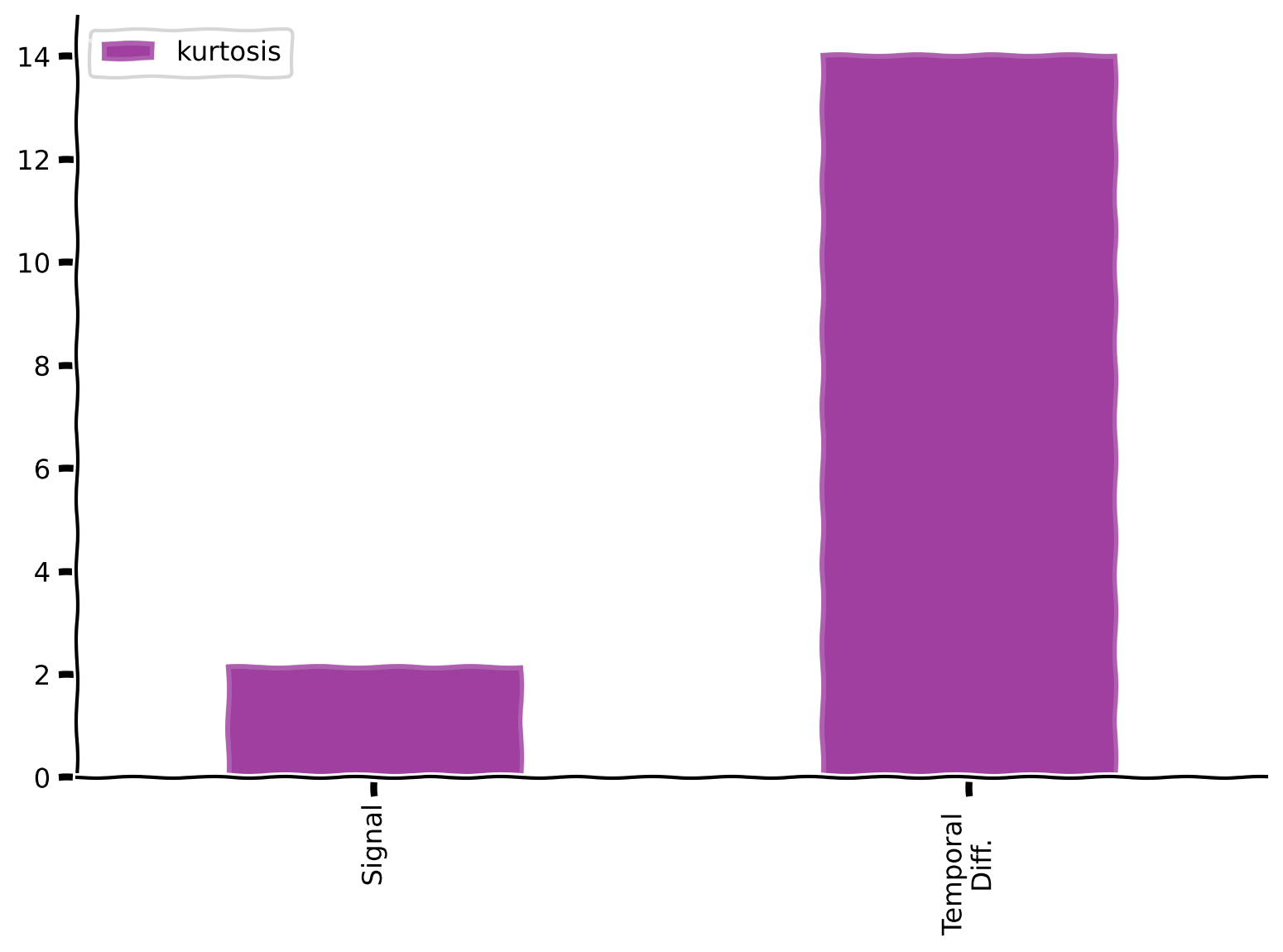
Coding Exercise 2.3: Changes over longer delays
What happens if we look at differences at longer delays ?
In this exercise, we will explore the effects of increasing values on the sparsity of the temporal differentiation signal.
Create an array of 10 different values: .
Create a list called taus_list composed of 10 arrays where each array is the temporal differentiation with a different interval .
Compare the histograms of temporal differences for each different tau. Plot these histograms together, with all histograms using the same bins.
Pay attention: here, it is NOT recommended to use the built-in np.diff function.
###################################################################
## Fill out the following then remove
raise NotImplementedError("Student exercise: complete calcualtion of `taus` and `taus_list`.")
###################################################################
num_taus = 10

# create taus
taus = np.linspace(1, 91, ...).astype(int)

# create taus_list
taus_list = [np.abs(sig[...:] - sig[:-tau]) for tau in taus]
---------------------------------------------------------------------------
NotImplementedError Traceback (most recent call last)
Cell In[17], line 3
1 ###################################################################
2 ## Fill out the following then remove
----> 3 raise NotImplementedError("Student exercise: complete calcualtion of `taus` and `taus_list`.")
4 ###################################################################
5 num_taus = 10
NotImplementedError: Student exercise: complete calcualtion of `taus` and `taus_list`.Plot your results
Source
# @title Plot your results
plot_temp_diff_histogram(sig, taus, taus_list)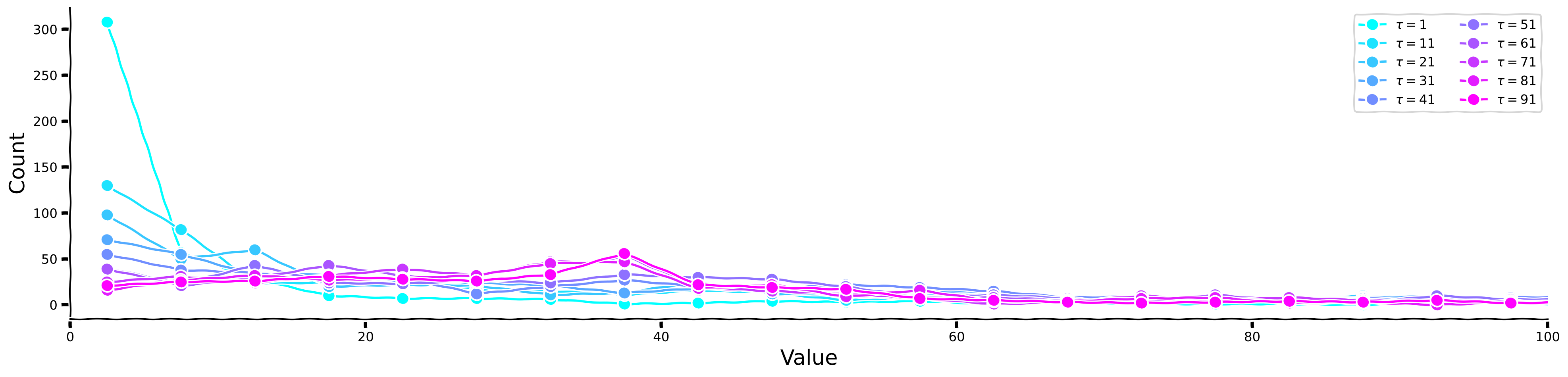
Now, let us look at the histograms for each separately, as well as for the kurtosis values.
Histogram plots for different values of 
Source
# @title Histogram plots for different values of $\tau$
plot_temp_diff_separate_histograms(sig, taus, taus_list)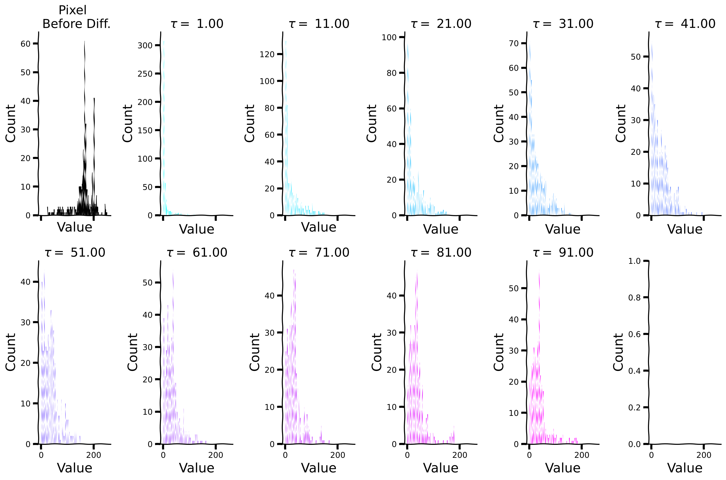
Plot sparsity (kurtosis) for different values of 
Source
# @title Plot sparsity (kurtosis) for different values of $\tau$
plot_temp_diff_kurtosis(sig, taus, taus_list)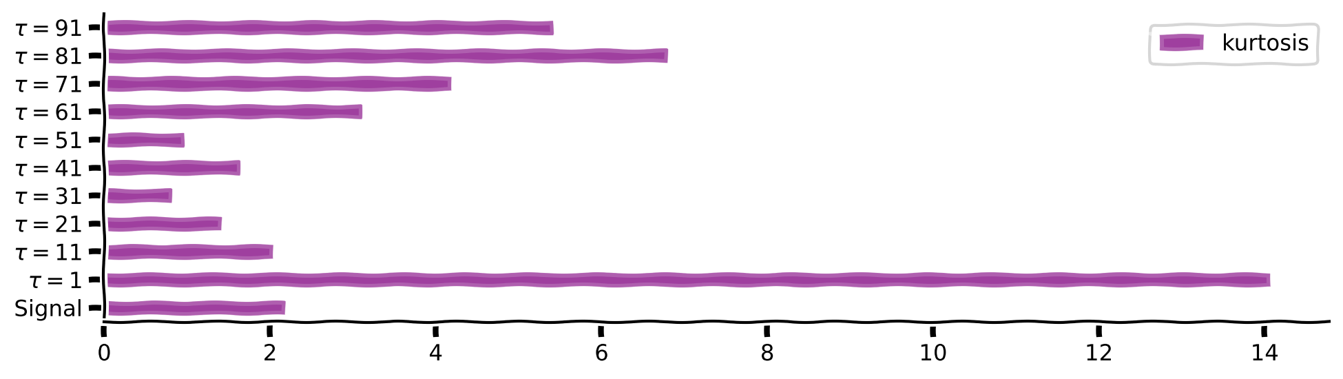
Exploring temporal differencing with a box filter
Instead of differences separated by delay , we’ll compute differences between one value and the average over a range of delays. This is closer to what brains actually do. Here we’ll use a box filter for the average.
We define a diff_box function, which accepts a signal and the window size as inputs. Internally, it computes the difference between the signal and the average signal over a delayed time window. Observe the results for window = 10. We will explore changes at different times scales by choosing different window sizes and then comparing the raw signal with its diff_box temporal derivatives for each size.
Filter visualization
Source
# @title Filter visualization

def diff_box(data, window, pad_size = 4):
    filter = np.concatenate([np.repeat(0,pad_size), np.repeat(0,window), np.array([1]), np.repeat(-1,window), np.repeat(0,pad_size)]).astype(float)
    filter /= np.sum(filter**2)**0.5

    filter_plus_sum =  filter[filter > 0].sum()
    filter_min_sum = np.abs(filter[filter < 0]).sum()
    filter[filter > 0] *= filter_min_sum/filter_plus_sum
    diff_box = np.convolve(data, filter, mode='full')[:len(data)]
    diff_box[:window] = diff_box[window]
    return diff_box, filter

window = 10
diff_box_signal, filter = diff_box(sig, window)

with plt.xkcd():
    fig, ax = plt.subplots()
    plot_e1 = np.arange(len(filter))
    plot_e2 = np.arange(len(filter)) + 1
    plot_edge_mean = 0.5*(plot_e1 + plot_e2)
    plot_edge = lists2list( [[e1 , e2] for e1 , e2 in zip(plot_e1, plot_e2)])
    ax.plot(plot_edge, np.repeat(filter, 2), alpha = 0.3, color = 'purple')
    ax.scatter(plot_edge_mean, filter, color = 'purple')
    add_labels(ax,ylabel = 'Filter Value', title = 'Box Filter', xlabel = 'Value')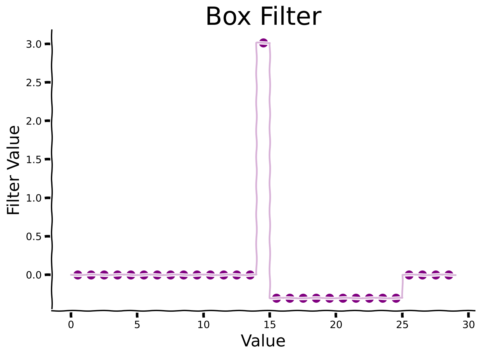
Discussion
Why do you think the filter is asymmetric?
How might a filter influence the sparsity patterns observed in data?
Plot signal and its temporal derivative on a longer timescale
Source
# @title Plot signal and its temporal derivative on a longer timescale
plot_diff_box(sig, filter, diff_box_signal)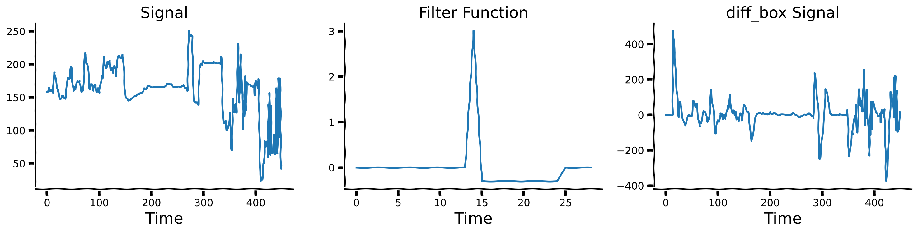
Now, we will define the window for 10 different values: windows = [1,11,21,...91] and calculate corresponding diff_box signal versions.
Define different window values
Source
# @title Define different window values
windows = np.linspace(1, 91, 10)
diff_box_values = [diff_box(sig, int(window))[0] for window in windows]
Visualize temporal differences for different window sizes
Source
# @title Visualize temporal differences for different window sizes

plot_diff_with_diff_box(sig, windows, diff_box_values)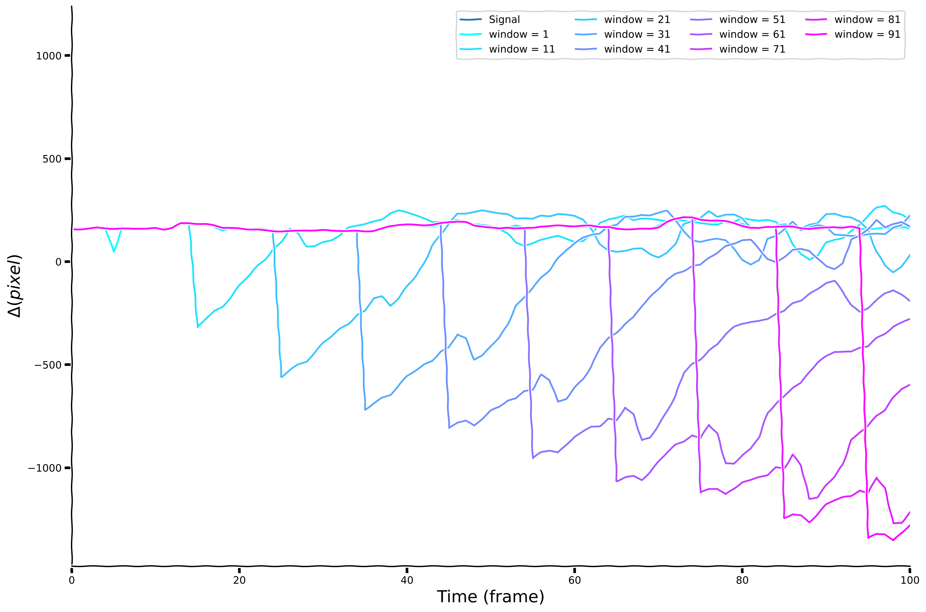
Histogram for each of the window size
Source
# @title Histogram for each of the window size

plot_temp_diff_separate_histograms(sig, windows, diff_box_values, tau = False)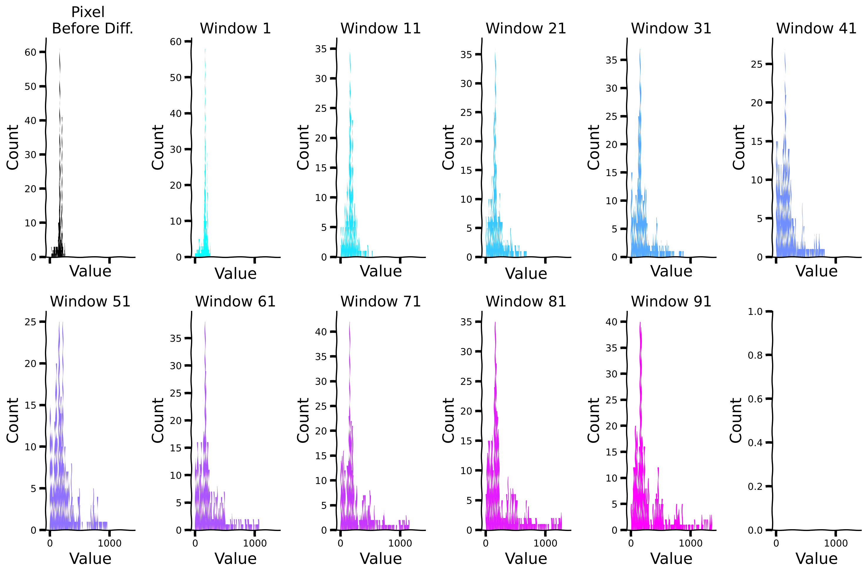
Compare sparsity (measured by kurtosis) for different window sizes
Source
# @title Compare sparsity (measured by kurtosis) for different window sizes

plot_temp_diff_kurtosis(sig, windows, diff_box_values, tau = False)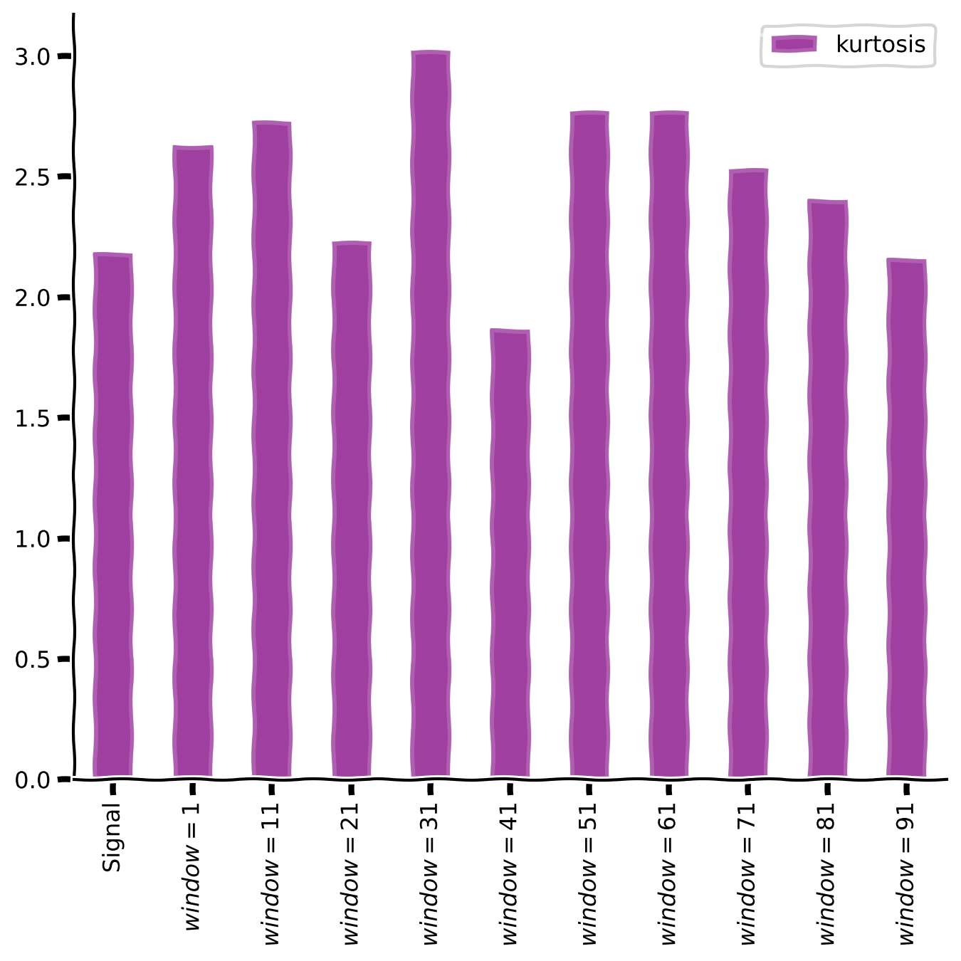
Discussion
What do you observe about the kurtosis after applying the temporal differentiation?
Section 3: Sparse coding
Estimated timing to here from start of tutorial: 35 minutes.
Sparse coding is a coding strategy where the inputs are represented by a linear combination of features, most with zero coefficients but a few that are nonzero or active. Often, this is applied with an overcomplete basis set: we use more features that are necessary to cover the input space. This concept is often applied to sensory inputs, such as images or sounds, where the goal is to find a concise and efficient representation that captures the essential features of the input.
In Section 3.1, we assume that the basis set is fixed and known, and we just want to find sparse coefficients (or activities) that best explain the input data.
In Section 3.2, we then describe how to find a good basis set for use in sparse coding.
Section 3.1: Finding coefficients for sparse codes
Video 4: Sparse coding
Neuroscience measures of sparse responses
In a pivotal experiment [1] at Johns Hopkins University, Hubel and Wiesel implanted an electrode into the visual cortex of a living cat and measured its electrical activity in response to displayed images.
Despite prolonged exposure to various images, no significant activity was recorded.
However, unexpectedly, when the slide was inserted and removed from the projector, the neurons responded robustly. This led to the discovery of neurons highly sensitive to edge orientation and location, providing the first insights into the type of information coded by neurons.
[1] Hubel DH, Wiesel TN (1962). “Receptive fields, binocular interaction and functional architecture in the cat’s visual cortex.” J. Physiol.160, 106-154.
Discussion
What implications do these specialized properties of neural representation hold for our understanding of visual perception?
How might these findings inform computational models of visual processing in artificial systems?
Computational Neuroscience model of sparse coding
In 1996, Olshausen and Field [2] demonstrated that sparse coding could be a good model of the early visual system, particularly in V1. They found that neuron selectivity in the visual cortex could be explained through sparse coding, where only a small subset of neurons responded to specific features or patterns. Receptive fields learned through this objective looked like orientation-specific edge detectors, like those in biological visual systems, as we will see below.
[2] Olshausen BA, Field DJ (1996). “Emergence of simple-cell receptive field properties by learning a sparse code for natural images.” Nature 381: 607-609.
pseudo-norm regularization to promote sparsity
The pseudo-norm is defined as the number of non-zero features in the signal. Particularly, let be a vector with “latent activity” features. Then:
Hence, the pseudo-norm can be used to promote sparsity by adding it to a cost function to “punish” the number of non-zero features.
Let’s assume that we have a simple linear model where we want to capture the observations using the linear model (which we will later call dictionary). ’s features (columns) can have sparse weights denoted by . This is known as a generative model, as it generates the sensory input.
For instance, in the brain, can represent a basis of neuronal networks while can capture their sparse time-changing contributions to the overall brain activity (e.g. see the dLDS model in [3]).
Hence, we are looking for the weights under the assumption that:
where is an i.i.d Gaussian noise with zero mean and std of , i.e., .
To enforce that is sparse, we penalize the number of non-zero features with penalty . We thus want to solve the following minimization problem:
[3] Mudrik, N., Chen, Y., Yezerets, E., Rozell, C. J., & Charles, A. S. (2024). Decomposed linear dynamical systems (dlds) for learning the latent components of neural dynamics. Journal of Machine Learning Research, 25(59), 1-44.
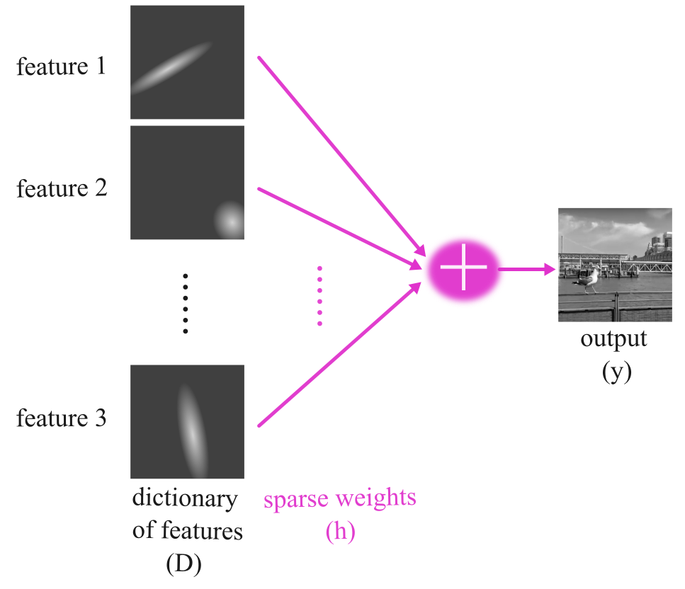
In the above figure and throughout this tutorial, we will use the following definitions:
: Dictionary
Features: Refers to the columns of (i.e., basis elements)
Basis: Refers to the collection of features
: A sparse vector assigning weights to the elements of
These definitions will help clarify the terminology used in discussing the concepts of dictionary learning and sparse coding.
How can we find the sparse vector given a dictionary?
One method to find a sparse solution for a linear decomposition with regularization is OMP (Orthogonal Matching Pursuit) [4]. As explained in the video, OMP is an approximate method to find the best matching features to represent a target signal.
OMP iteratively selects the features that best correlate with the remaining part of the signal, updates the remaining part by subtracting the contribution of the chosen features, and repeats until the remaining part is minimized or the desired number of features is selected.
In this context, a “dictionary” is a collection of features that we use to represent the target signal. These features are like building blocks, and the goal of the OMP algorithm is to find the right combination of these blocks from the dictionary to match the target signal best.
[4] Pati, Y. C., Rezaiifar, R., & Krishnaprasad, P. S. (1993, November). “Orthogonal matching pursuit: Recursive function approximation with applications to wavelet decomposition.” In Proceedings of 27th Asilomar conference on signals, systems, and computers (pp. 40-44). IEEE.
Coding Exercise 3: OMP algorithm
Now, we will explore the Orthogonal Matching Pursuit (OMP) algorithm with increasing sparsity levels and examine how pixel values are captured by different frequencies.
We will follow the following steps:
Generate sinusoidal features with varying frequencies ranging from 0.001 to 1, applying each frequency to a time array. These features will serve in this exercise as the dictionary.
Implement the OMP algorithm with increasing sparsity levels. Feel free to change the number of non-zero coefficients (in
n_nonzero_coefsto explore its effect.Fit the generated sinusoidal signals to the dictionary of frequencies you defined.
Evaluate how well each sparsity level captures the variations in features.
Explore the results to understand the trade-off between sparsity and the accuracy of signal representation.
###################################################################
## Fill out the following then remove
raise NotImplementedError("Student exercise: complete OMP algorithm preparation.")
###################################################################
T_ar = np.arange(len(sig))

#100 different frequency values from 0.001 to 1, then apply each frequency on `T_ar`
freqs = np.linspace(0.001, 1, ...)
set_sigs = [np.sin(...*...) for f in freqs]

# define 'reg' --- an sklearn object of OrthogonalMatchingPursuit, and fit it to the data, where the frequency bases are the features and the signal is the label
reg = OrthogonalMatchingPursuit(fit_intercept = True, n_nonzero_coefs = 10).fit(np.vstack(set_sigs).T, sig)
---------------------------------------------------------------------------
NotImplementedError Traceback (most recent call last)
Cell In[27], line 3
1 ###################################################################
2 ## Fill out the following then remove
----> 3 raise NotImplementedError("Student exercise: complete OMP algorithm preparation.")
4 ###################################################################
5 T_ar = np.arange(len(sig))
NotImplementedError: Student exercise: complete OMP algorithm preparation.Observe the plot of 3 example signals.
Plot of 3 basis signals
Source
# @title Plot of 3 basis signals

with plt.xkcd():
    fig, axs = plt.subplots(3,1,sharex = True, figsize = (10,5), sharey = True)
    axs[0].plot(set_sigs[0], lw = 3)
    axs[1].plot(set_sigs[1], lw = 3)
    axs[2].plot(set_sigs[-1], lw = 3)
    [remove_edges(ax) for ax in axs]
    [ax.set_xlim(left = 0) for ax in axs]
    fig.tight_layout()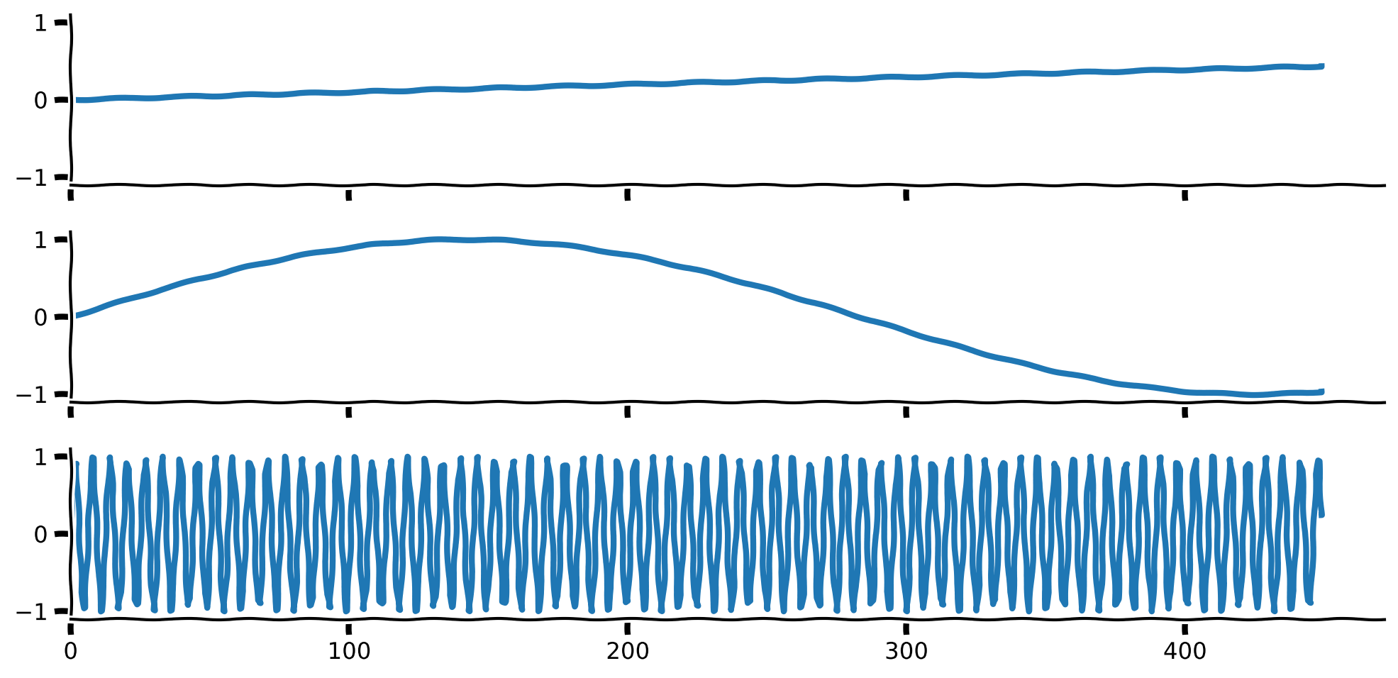
Next, run the following code to plot the basis features and the reconstruction.
Visualize basis features and signal reconstruction
Source
# @title Visualize basis features and signal reconstruction

with plt.xkcd():
    fig, axs = plt.subplots(2,2, figsize = (15,10))
    axs = axs.flatten()

    sns.heatmap(np.vstack(set_sigs), ax = axs[0])
    axs[0].set_yticks(np.arange(0,len(freqs)-.5, 4)+ 0.5)
    axs[0].set_yticklabels(['$f = %.4f$'%freqs[int(j)] for j in np.arange(0,len(freqs)-0.5, 4)], rotation = 0)
    add_labels(axs[0], xlabel = 'Time', ylabel= 'Basis Features', title = 'Frequency Basis Features')

    axs[1].plot(sig, label = 'Original', lw = 4)
    axs[1].plot(reg.predict(np.vstack(set_sigs).T), lw = 4, label = 'Reconstruction')
    remove_edges(axs[1])
    axs[1].legend()
    add_labels(axs[1], xlabel = 'Time', ylabel= 'Signal', title = 'Reconstruction')
    axs[1].set_xlim(left = 0)

    axs[2].stem(freqs, reg.coef_)
    remove_edges(axs[2])
    add_labels(axs[2], xlabel = 'Frequencies', ylabel= 'Frequency weight', title = 'Frequency Components Contributions')
    axs[2].set_xlim(left = 0)

    num_colors = np.sum(reg.coef_ != 0)
    cmap_name = 'winter'
    samples = np.linspace(0, 1, num_colors)
    colors = plt.colormaps[cmap_name](samples)
    colors_expand = np.zeros((len(reg.coef_), 4))
    colors_expand[reg.coef_!= 0] = np.vstack(colors)

    axs[-1].plot(sig, label = 'Original', color = 'black')
    [axs[-1].plot(reg.coef_[j]*set_sigs[j] + reg.intercept_, label = '$f = %.4f$'%f, lw = 4, color = colors_expand[j]) for j, f in enumerate(freqs) if  reg.coef_[j] != 0]
    remove_edges(axs[-1])
    axs[-1].legend(ncol = 4)
    axs[-1].set_xlim(left = 0)
    add_labels(axs[-1], xlabel = 'Time', ylabel= 'Signal', title = 'Contribution')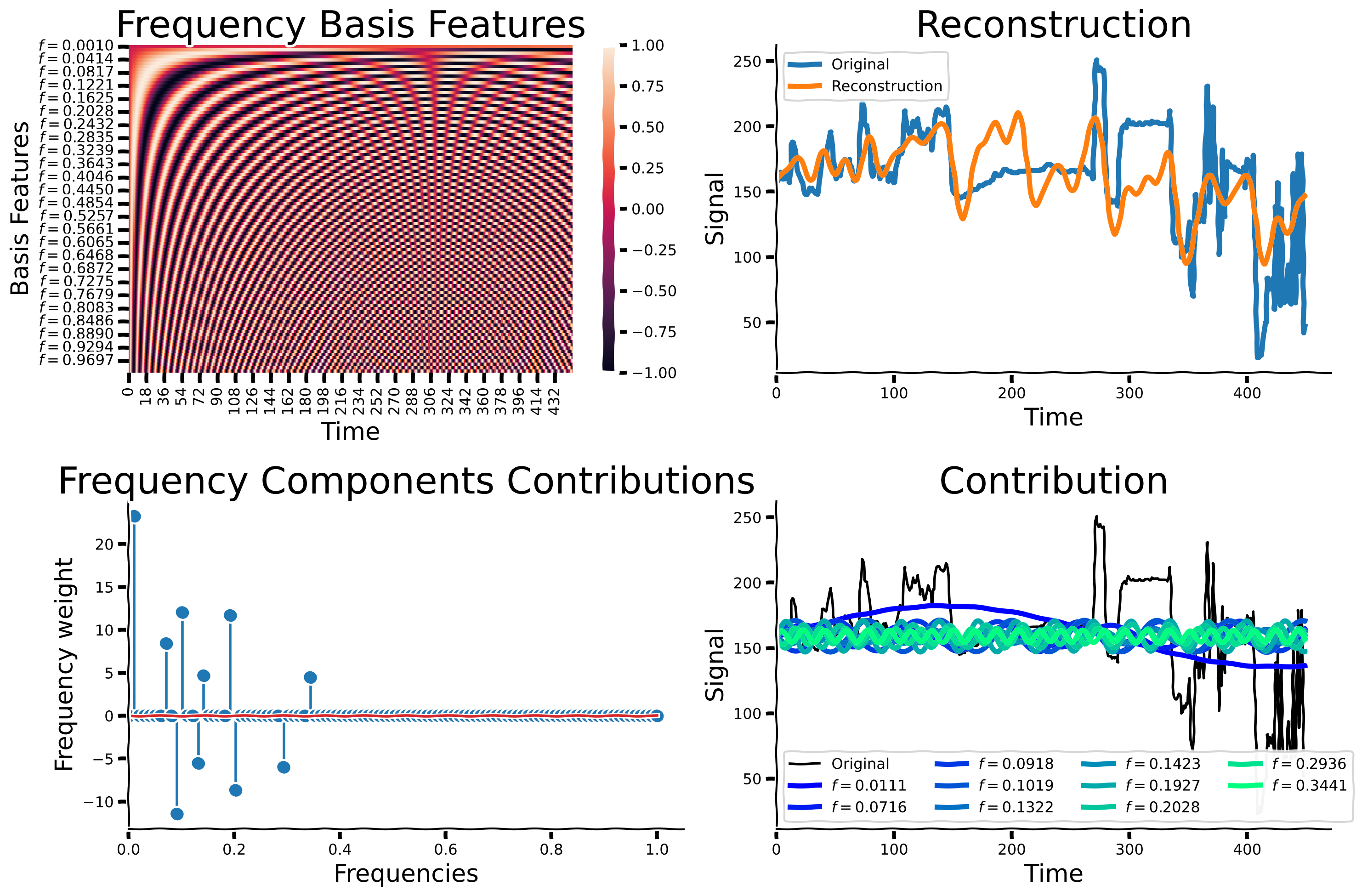
Now, we will explore the effect of increasing the number of non-zero coefficients. We define the number of non-zero coefficients to be the cardinality. Below, please run OMP with increasing numbers of non-zero coefficients (increasing cardinality), from 1 to 101 in intervals of 5. We will then compare the accuracy and reconstruction performance of each fitted model to exmamine the relationship between cardinality and signal reconstruction. You should already have an idea what the performance might look like when considering a very low cardinality and a very high cardinality. If you are familiar with dimensionality reduction techniques like PCA, this should give you a starting point to frame this question.
OMP for different cardinality
Source
# @title OMP for different cardinality

# define a list or numpy array of optional cardinalities from 1 to 51 in intervals of 5.
cardinalities = np.arange(1,101,5)

# For each of the optional cardinalities, run OMP using the pixel's signal from before. Create a list called "regs" that includes all OMP's fitted objects
regs = [OrthogonalMatchingPursuit(fit_intercept = True, n_nonzero_coefs = card).fit(np.vstack(set_sigs).T, sig) for card in cardinalities]
Now, let’s observe the effect of the cardinality on the reconstruction.
Cardinality impact on reconstruction quality
Source
# @title Cardinality impact on reconstruction quality

with plt.xkcd():
    fig, axs = plt.subplots(1, 2, figsize = (15,5))
    ax = axs[0]
    ax.plot(cardinalities, [reg.score(np.vstack(set_sigs).T, sig) for reg in regs], marker = '.')

    ax.set_xlim(left = 0)
    ax.set_ylim(bottom = 0)
    add_labels(ax, ylabel = 'coefficient of determination', xlabel  = 'Cardinality')
    remove_edges(ax)
    mean_er = np.vstack([np.mean((reg.predict(np.vstack(set_sigs).T) - sig)**2)**0.5 for reg in regs])

    axs[1].plot(cardinalities, mean_er)
    axs[1].set_xlim(left = 0)
    axs[1].set_ylim(bottom = 0)
    remove_edges(axs[1])
    add_labels(axs[1], ylabel = 'rMSE', xlabel  = 'Cardinality')
    plt.show()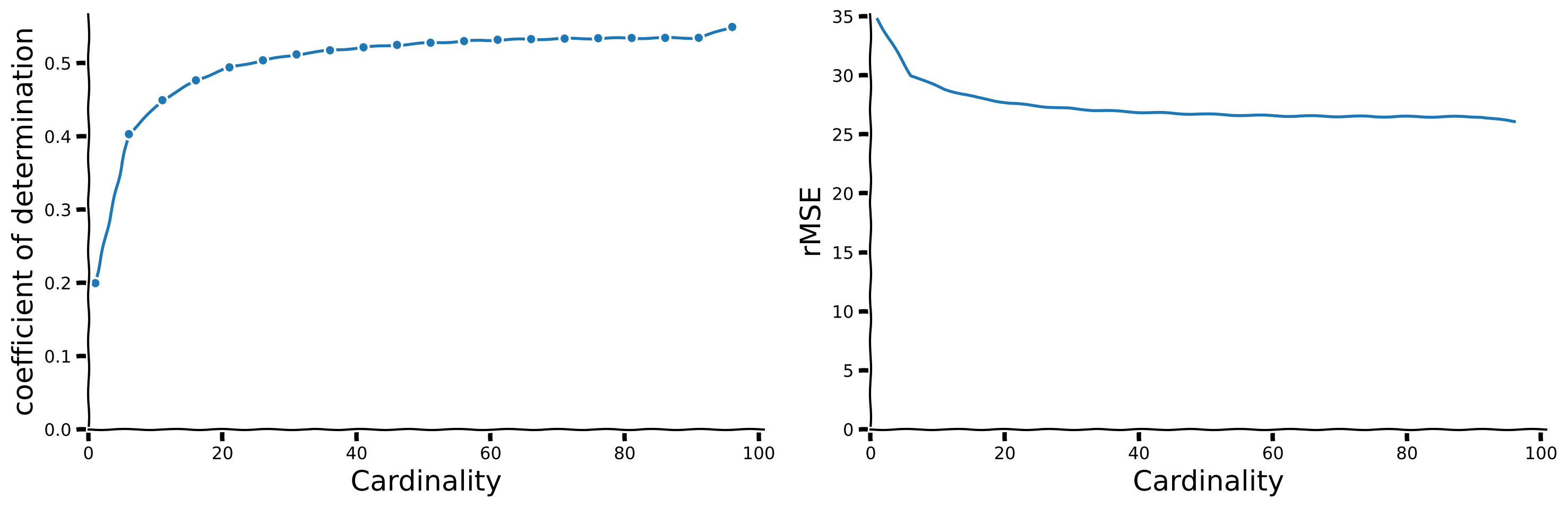
How would you choose the ideal cardinality?
Hint: Look for an ‘ankle’ in complexity vs. sparsity plots, which indicates a balance between expressivity and sparsity. Discuss these observations with your group to determine the most effective cardinality.
How does the above affect generalization?
Hint: Consider how learning fewer but most relevant features from noisy data might help the model generalize better to new, unseen data.
What is your conclusion?
Hint: Discuss how sparsity, which emphasizes few significant features, improves the model’s robustness and utility in real-world scenarios and the considerations needed when setting the level of sparsity.
Challenges with OMP
While OMP is a common and simple practice for finding the sparse representation of a dictionary of features, it presents multiple challenges. The norm is not convex, making it hard to identify the sparse vector. Another challenge is computational complexity. Approaches addressing these issues exist. Some of them replace the norm with its approximation, promoting sparsity while retaining convexity, making it easier to optimize.
Section 3.2: Hidden features as dictionary learning
Estimated timing to here from start of tutorial: 55 minutes.
Video 5: Dictionary learning
What if we do not know the dictionary of features?
In OMP, we’ve assumed that we already know the features and are solely focused on identifying which sparse combination can best describe the data. However, in real-world scenarios, we frequently lack knowledge about the fundamental components underlying the data. In other words, we don’t know the features and must learn them.
Dictionary Learning: To address this problem, Dictionary Learning aims to simultaneously learn both the dictionary of features and the sparse representation of the data. It iteratively updates the dictionary and the sparse codes until convergence, typically minimizing a reconstruction error term along with a sparsity-inducing regularizer.
How is it related to the brain? Dictionary Learning draws parallels to the visual system’s ability to extract features from raw sensory input. In the brain, the visual system processes raw visual stimuli through hierarchical layers, extracting increasingly complex features at each stage. Similarly, Dictionary Learning aims to decompose complex data into simpler components, akin to how the visual system breaks down images into basic visual features like edges and textures.
Now, let’s apply Dictionary Learning to various types of data to unveil the latent components underlying it.
Coding Exercise 4: Dictionary Learning for MNIST
In this exercise, we first load a new short video created from MNIST images, as shown below. We then use sklearn’s DictionaryLearning to find the dictionary’s () features.
In particular, we will follow the following steps:
Load the Video Data: Begin by loading the 3D video data from the
reweight_digits.npyfile, which contains pixel data over time. The video is shown in the above video from 2:34, which depicts an evolving transition of MNIST digits over time.Preprocess the Video Data: Create a copy of the video data to work on without altering the original data. Extract the total number of frames, as well as the dimensions of each frame, adjusting for any specific modifications (e.g., reducing the width by 10 columns).
Prepare Frames for Analysis: Flatten each frame of the video to convert the 2D image data into 1D vectors. Store these vectors in a list, which is then converted into a NumPy array for efficient processing.
Initialize Dictionary Learning: Set up a dictionary learning model with specific parameters (e.g., number of components, the algorithm for transformation, regularization strength, and random state for reproducibility).
Fit and Transform the Data (YOUR EXERCISE): Fit the dictionary learning model to the prepared video data and transform it to obtain sparse representations. This involves completing the implementation of
dict_learner.fit(...).transform(...)by providing the necessary input arguments based on your tutorial’s context. Pay attention, as usual, you will need to remove the placeholderraise NotImplementedErrorand replace it with the appropriate function call tofitandtransformthe data.
###################################################################
## Fill out the following then remove.
raise NotImplementedError("Student exercise: complete calcualtion of `D_transformed`.")
###################################################################

# Video_file is a 3D array representing pixels X pixels X time
video_file = np.load('reweight_digits.npy')

# Create a copy of the video_fire array
im_focus = video_file.copy()

# Get the number of frames in the video
T = im_focus.shape[2]

# Get the number of rows in the video
N0 = im_focus.shape[0]

# Get the number of columns in the video, leaving out 10 columns
N1 = im_focus.shape[1] - 10

# Create a copy of the extracted frames
low_res = im_focus.copy()

# Get the shape of a single frame
shape_frame = low_res[:, :, 0].shape

# Flatten each frame and store them in a list
video_file_ar = [low_res[:, :, frame].flatten() for frame in range(low_res.shape[2])]

# Create dict_learner object
dict_learner = DictionaryLearning(
    n_components=15, transform_algorithm='lasso_lars', transform_alpha=0.9,
    random_state=402,
)

# List to np.array
video_v = np.vstack(video_file_ar)

# Fit and transform `video_v`
D_transformed = dict_learner.fit(...).transform(...)
---------------------------------------------------------------------------
NotImplementedError Traceback (most recent call last)
Cell In[32], line 3
1 ###################################################################
2 ## Fill out the following then remove.
----> 3 raise NotImplementedError("Student exercise: complete calcualtion of `D_transformed`.")
4 ###################################################################
5
6 # Video_file is a 3D array representing pixels X pixels X time
7 video_file = np.load('reweight_digits.npy')
NotImplementedError: Student exercise: complete calcualtion of `D_transformed`.Let’s visualize the identified features!
Visualization of features
Source
# @title Visualization of features

with plt.xkcd():
    num_thetas = 20
    cmap_name = 'plasma'
    samples = np.linspace(0, 1, len(dict_learner.components_)+1)
    colors = plt.colormaps[cmap_name](samples)

    num_comps = len(dict_learner.components_)

    fig, axs = plt.subplots(2, int((1+num_comps)/2) , figsize = (16,4), sharey = True, sharex = True)
    axs = axs.flatten()
    [sns.heatmap(dict_learner.components_[j].reshape(shape_frame), square = True, cmap ='gray', robust = True, ax = axs[j]) for j in range(num_comps)]
    titles = ['Atom %d'%j for j in range(1, num_comps +1)]
    [ax.set_title(title, color = colors[j], fontsize = 10)
    for j, (title, ax) in enumerate(zip(titles, axs))]
    axs[-1].set_visible(False)
---------------------------------------------------------------------------
NameError Traceback (most recent call last)
Cell In[33], line 6
4 num_thetas = 20
5 cmap_name = 'plasma'
----> 6 samples = np.linspace(0, 1, len(dict_learner.components_)+1)
7 colors = plt.colormaps[cmap_name](samples)
9 num_comps = len(dict_learner.components_)
NameError: name 'dict_learner' is not definedVisualization of impact of features through the time
Source
# @title Visualization of impact of features through the time

D = np.linalg.pinv(dict_learner.components_.T) @ video_v.T
D_transformed_norm = D.T.copy()
with plt.xkcd():
    fig, ax = plt.subplots(figsize = (16,3))
    [ax.plot(D_transformed_norm[:,j], color = colors[j], lw = 5, label = 'Atom %d'%(j+1))
     for j in range(num_comps)]
    remove_edges(ax)
    ax.set_xlim(left = 0)
    [ax.set_yticks([]) for ax in axs]
    [ax.set_xticks([]) for ax in axs]

    add_labels(ax, xlabel = 'Time', ylabel = 'Coefficients', title = 'Features Ceofficients')
    create_legend({'Atom %d'%(j+1): colors[j] for j in range(num_comps)},
                  params_leg = {'ncol': 3})
---------------------------------------------------------------------------
NameError Traceback (most recent call last)
Cell In[34], line 3
1 # @title Visualization of impact of features through the time
----> 3 D = np.linalg.pinv(dict_learner.components_.T) @ video_v.T
4 D_transformed_norm = D.T.copy()
5 with plt.xkcd():
NameError: name 'dict_learner' is not definedNow, let’s compare the components to PCA.
PCA components visualization
Source
# @title PCA components visualization

data_mat = np.vstack(video_file_ar)
# Assuming your data is stored in a variable named 'data_mat' (N by p numpy array)
# where N is the number of samples and p is the number of features

# Create a PCA object with 20 components
pca = PCA(n_components=15)

# Fit the PCA model to the data
pca.fit(data_mat)

# Access the 20 PCA components
pca_components = pca.components_

pca_componens_images = [pca_components[comp,:].reshape(shape_frame) for comp in range(num_comps)]

with plt.xkcd():
    fig, axs = plt.subplots(2, int((1+num_comps)/2) , figsize = (16,4), sharey = True, sharex = True)
    axs = axs.flatten()
    [sns.heatmap(im, ax = axs[j], square = True, cmap ='gray', robust = True) for j,im in enumerate(pca_componens_images)]
    titles = ['Atom %d'%j for j in range(1, num_comps +1)]
    [ax.set_title(title, color = colors[j], fontsize = 10) for j, (title, ax) in enumerate(zip(titles, axs))]
    axs[-1].set_visible(False)
---------------------------------------------------------------------------
NameError Traceback (most recent call last)
Cell In[35], line 3
1 # @title PCA components visualization
----> 3 data_mat = np.vstack(video_file_ar)
4 # Assuming your data is stored in a variable named 'data_mat' (N by p numpy array)
5 # where N is the number of samples and p is the number of features
6
7 # Create a PCA object with 20 components
8 pca = PCA(n_components=15)
NameError: name 'video_file_ar' is not definedSection 4: Identifying sparse visual fields in natural images using sparse coding
Estimated timing to here from start of tutorial: 1 hour 5 minutes.
In this section we will understand the basis of visual field perception.
Video 6: Sparse visual fields
Dictionary Learning for CIFAR10
We will use the CIFAR10 dataset. Let’s, at first, load the data.
Load CIFAR-10 dataset
Source
# @title Load CIFAR-10 dataset

import contextlib
import io

with contextlib.redirect_stdout(io.StringIO()): #to suppress output
    (x_train, y_train), (x_test, y_test) = tf.keras.datasets.cifar10.load_data()
Now, let’s create a short video of these images switching. Now, we will detect the underlying visual fields.
Create & explore video
Source
# @title Create & explore video

num_image_show = 50
img_index = np.random.randint(0, len(x_train), num_image_show)
x_train_ar = np.copy(x_train)[img_index]
video_gray = 0.2989 * x_train_ar[:, :, :,0] + 0.5870 * x_train_ar[:, :, :,1] + 0.1140 * x_train_ar[:, :, :,2]

def show_slice_CIFAR(slice_index):
    with plt.xkcd():
        plt.figure(figsize=(2, 2))
        plt.imshow(data_CIFAR[slice_index] , cmap='gray')
        plt.axis('off')
        plt.show()

data_CIFAR = np.repeat(video_gray, 1, axis = 0)

# Create a slider to select the slice
slider = IntSlider(min=0, max=data_CIFAR.shape[0] - 1, step=1, value=0, description='Frame')

# Connect the slider and the function
interact(show_slice_CIFAR, slice_index=slider)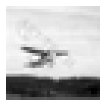
<function __main__.show_slice_CIFAR(slice_index)>Now, let’s try to extract the visual field from the images. Look at the components identified below and compare the ones identified by PCA to those identified by Olshausen & Field via sparse dictionary learning.
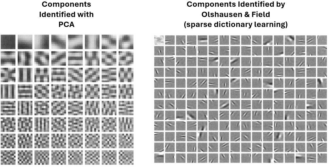
Following Olshausen & Field’s paper, we will demonstrate how to receive visual field components that emerge from real-world images.
We expect to find features that are:
Spatially localized.
Oriented.
Selective to structure at different spatial scales.
We would like to understand the receptive field properties of neurons in the visual cortex by applying sparsity to identify the basic fundamental components underlying natural images.
We will reshape the CIFAR data we loaded before so that the time (frame) axis is the last one.
video_file = data_CIFAR.transpose((1,2,0))For the exercise, we will focus on a small subset of the data so that you can understand the idea. We will later load better results trained for a longer time.
We will first set some parameters to take a small subset of the video. In the cell below, you can explore parameters that are set by default.
Set default parameters
Source
# @title Set default parameters

size_check =  4 # 32 for the full size

# how many images we want to consider? (choose larger numbers for better results)
num_frames_include =  80

# set number of dictionary features
dict_comp = 8

# set number of model iterations
max_iter = 100

num_frames_include = np.min([num_frames_include , x_train.shape[0]])
Let’s visualize the small subset we are taking for the training.
Images visualization
Source
# @title Images visualization

# let's choose some random images to focus on
img_index = np.random.randint(0, len(x_train), num_frames_include)
x_train_ar = np.copy(x_train)[img_index]

# change to grayscale
video_gray = 0.2989 * x_train_ar[:, :, :,0] + 0.5870 * x_train_ar[:, :, :,1] + 0.1140 * x_train_ar[:, :, :,2]

# update data and create short movie
data_CIFAR = np.repeat(video_gray, 1, axis = 0)

# Create a slider to select the slice
slider = IntSlider(min=0, max=data_CIFAR.shape[0] - 1, step=1, value=0, description='Frame')

# Connect the slider and the function
interact(show_slice_CIFAR, slice_index=slider)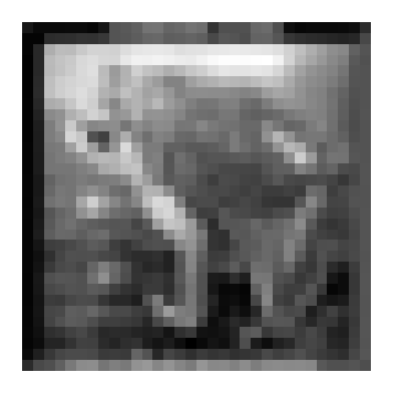
<function __main__.show_slice_CIFAR(slice_index)>Coding Exercise 5: Find the latent components by training the dictionary learner
Training time will take around 1 minute.
Please follow the following steps:
Choose Alpha ():
Each group member should select a unique value for between approximately ~0.0001 and ~1.
controls the sparsity of the learned dictionary components in the DictionaryLearning algorithm.
Discussion: Before running the model, discuss your expectations on how different values might affect the sparsity and quality of learned features.
Apply Dictionary Learning:
Use the chosen to fit the DictionaryLearning model (
dict_learner).Compare and document how each (selected by different group members) influences the sparsity and quality of learned dictionary components. Note: Each member should choose only one due to computational constraints.
Visualize Results:
Plot heatmap visualizations (
sns.heatmap) to examine individual dictionary components for each value.Plot coefficients over time (
D_transformed) to analyze and compare how they vary across different values.
Group Discussion:
Compare your results with peers who selected different values.
Discuss and interpret the impact of on sparsity and feature representation.
Summarize findings on which values appear most effective for achieving desired sparsity and representation quality.
# Get the number of frames in the video
T = video_file.shape[2]

# Get the number of rows in the video
N0 = video_file.shape[0]

# Get the number of columns in the video, leaving out 10 columns
N1 = video_file.shape[1] - 10

# Get the shape of a single frame
shape_frame = video_file[:, :, 0].shape

# Flatten each frame and store them in a list
num_frames_include = np.min([num_frames_include, video_file.shape[2]])

size_check = np.min([size_check, video_file.shape[0]])

video_file_ar = [video_file[:size_check, :size_check, frame].flatten() for frame in range(num_frames_include)]

###################################################################
## Fill out the following then remove.
raise NotImplementedError("Student exercise: please choose an $\alpha$ value here. Recommended $0.0001 <= \alpha <= 1$")
###################################################################

alpha = ...

dict_learner = DictionaryLearning(
    n_components=dict_comp, transform_algorithm = 'lasso_lars', transform_alpha=alpha,
    random_state=42,
)

D_transformed = dict_learner.fit_transform(np.vstack(video_file_ar))

with plt.xkcd():
    num_rows = 3
    num_cols =  int(( num_frames_include + 2)/num_rows)
    shape_frame = (size_check,size_check)

    cmap_name = 'plasma'
    samples = np.linspace(0, 1, len(dict_learner.components_)+1)
    colors = plt.colormaps[cmap_name](samples)
    num_comps = len(dict_learner.components_)

    vmin =  np.min(np.vstack(dict_learner.components_))
    vmax = np.max(np.vstack(dict_learner.components_))


    [sns.heatmap(dict_learner.components_[j].reshape(shape_frame), ax = axs[j], square = True, vmin = vmin, vmax = vmax,
                  cmap = 'PiYG', center = 0, cbar = False)  for j in range(num_comps)]

    [ax.set_xticks([]) for ax in axs]
    [ax.set_yticks([]) for ax in axs]

    titles = ['Atom %d'%j for j in range(1, num_comps +1)];
    [ax.set_title(title,  fontsize = 40) for j, (title, ax) in enumerate(zip(titles, axs))]


    fig, ax = plt.subplots(figsize = (20,5))
    [ax.plot(D_transformed[:,j],  lw = 5, label = 'Atom %d'%(j+1))
      for j in range(num_comps)]
    remove_edges(ax)
    ax.set_xlim(left = 0)
    [ax.set_yticks([]) for ax in axs]
    [ax.set_xticks([]) for ax in axs]

    add_labels(ax, xlabel = 'Time', ylabel = 'Coefficients', title = "Features' Coefficients")
    fig.tight_layout()
---------------------------------------------------------------------------
NotImplementedError Traceback (most recent call last)
Cell In[41], line 22
18 video_file_ar = [video_file[:size_check, :size_check, frame].flatten() for frame in range(num_frames_include)]
20 ###################################################################
21 ## Fill out the following then remove.
---> 22 raise NotImplementedError("Student exercise: please choose an $\alpha$ value here. Recommended $0.0001 <= \alpha <= 1$")
23 ###################################################################
25 alpha = ...
NotImplementedError: Student exercise: please choose an $lpha$ value here. Recommended $0.0001 <= lpha <= 1$# Get the number of frames in the video
T = video_file.shape[2]
# Get the number of rows in the video
N0 = video_file.shape[0]
# Get the number of columns in the video, leaving out 10 columns
N1 = video_file.shape[1] - 10
# Get the shape of a single frame
shape_frame = video_file[:, :, 0].shape
# Flatten each frame and store them in a list
num_frames_include = np.min([num_frames_include, video_file.shape[2]])
size_check = np.min([size_check, video_file.shape[0]])
video_file_ar = [video_file[:size_check, :size_check, frame].flatten() for frame in range(num_frames_include)]
alpha = 0.5
dict_learner = DictionaryLearning(
n_components=dict_comp, transform_algorithm = 'lasso_lars', transform_alpha=alpha,
random_state=42,
)
D_transformed = dict_learner.fit_transform(np.vstack(video_file_ar))
with plt.xkcd():
num_rows = 3
num_cols = int(( num_frames_include + 2)/num_rows)
shape_frame = (size_check,size_check)
cmap_name = 'plasma'
samples = np.linspace(0, 1, len(dict_learner.components_)+1)
colors = plt.colormaps[cmap_name](samples)
num_comps = len(dict_learner.components_)
vmin = np.min(np.vstack(dict_learner.components_))
vmax = np.max(np.vstack(dict_learner.components_))
[sns.heatmap(dict_learner.components_[j].reshape(shape_frame), ax = axs[j], square = True, vmin = vmin, vmax = vmax,
cmap = 'PiYG', center = 0, cbar = False) for j in range(num_comps)]
[ax.set_xticks([]) for ax in axs]
[ax.set_yticks([]) for ax in axs]
titles = ['Atom %d'%j for j in range(1, num_comps +1)];
[ax.set_title(title, fontsize = 40) for j, (title, ax) in enumerate(zip(titles, axs))]
fig, ax = plt.subplots(figsize = (20,5))
[ax.plot(D_transformed[:,j], lw = 5, label = 'Atom %d'%(j+1))
for j in range(num_comps)]
remove_edges(ax)
ax.set_xlim(left = 0)
[ax.set_yticks([]) for ax in axs]
[ax.set_xticks([]) for ax in axs]
add_labels(ax, xlabel = 'Time', ylabel = 'Coefficients', title = "Features' Coefficients")
fig.tight_layout()---------------------------------------------------------------------------
IndexError Traceback (most recent call last)
Cell In[42], line 44
40 vmin = np.min(np.vstack(dict_learner.components_))
41 vmax = np.max(np.vstack(dict_learner.components_))
---> 44 [sns.heatmap(dict_learner.components_[j].reshape(shape_frame), ax = axs[j], square = True, vmin = vmin, vmax = vmax,
45 cmap = 'PiYG', center = 0, cbar = False) for j in range(num_comps)]
47 [ax.set_xticks([]) for ax in axs]
48 [ax.set_yticks([]) for ax in axs]
Cell In[42], line 44, in <listcomp>(.0)
40 vmin = np.min(np.vstack(dict_learner.components_))
41 vmax = np.max(np.vstack(dict_learner.components_))
---> 44 [sns.heatmap(dict_learner.components_[j].reshape(shape_frame), ax = axs[j], square = True, vmin = vmin, vmax = vmax,
45 cmap = 'PiYG', center = 0, cbar = False) for j in range(num_comps)]
47 [ax.set_xticks([]) for ax in axs]
48 [ax.set_yticks([]) for ax in axs]
IndexError: index 2 is out of bounds for axis 0 with size 2Due to our efforts to limit computation time, we focused on a small area of the images, and we only considered a limited number of them with a restricted number of iterations. As a result, the quality of the outcomes was poor. For your exploration, we are providing better results obtained from training on a larger amount of images. This is important for discovering the components that better resemble the biological visual field.
Load full model & visualize features
Source
# @title Load full model & visualize features
res = np.load('model.npy', allow_pickle = True).item()
comps = res['dict_learner_components_']

with plt.xkcd():
    shape_frame = (32,32)

    cmap_name = 'plasma'
    samples = np.linspace(0, 1, len(comps)+1)
    colors = plt.colormaps[cmap_name](samples)
    num_comps = len(comps)

    vmin =  np.min(np.vstack(comps))
    vmax = np.max(np.vstack(comps))

    fig, axs = plt.subplots(2, int(np.ceil((num_comps+1)/2)) , figsize = (20,15), sharey = True, sharex = True)
    axs = axs.flatten()


    [axs[j].imshow(comps[j].reshape(shape_frame), vmin = 0)  for j in range(num_comps)]

    [ax.set_xticks([]) for ax in axs]
    [ax.set_yticks([]) for ax in axs]

    titles = ['Atom %d'%j for j in range(1, num_comps +1)];
    [ax.set_title(title,  fontsize = 40, color = colors[j]) for j, (title, ax) in enumerate(zip(titles, axs))]
    axs[-1].set_visible(False)
    axs[-2].set_visible(False)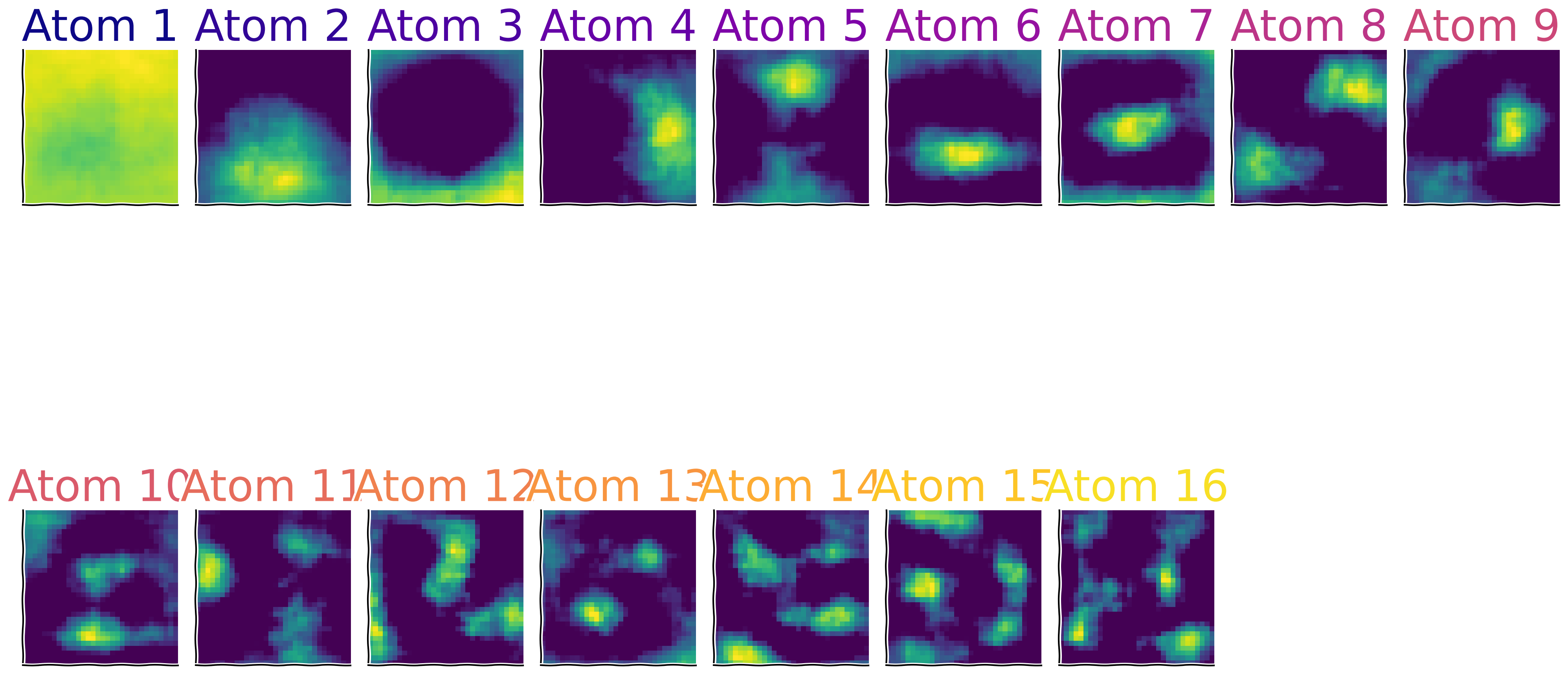
Sparse Activity of the components ()
Source
# @title Sparse Activity of the components ($h$)
D_transformed = res['X_transformed']
with plt.xkcd():
fig, ax = plt.subplots(figsize = (20,5))
[ax.plot(D_transformed[:,j], color = colors[j], lw = 5, label = 'Atom %d'%(j+1))
for j in range(num_comps)]
remove_edges(ax)
ax.set_xlim(left = 0)
[ax.set_yticks([]) for ax in axs]
[ax.set_xticks([]) for ax in axs]
add_labels(ax, xlabel = 'Time', ylabel = 'Coefficients', title = "Features' Coefficients")
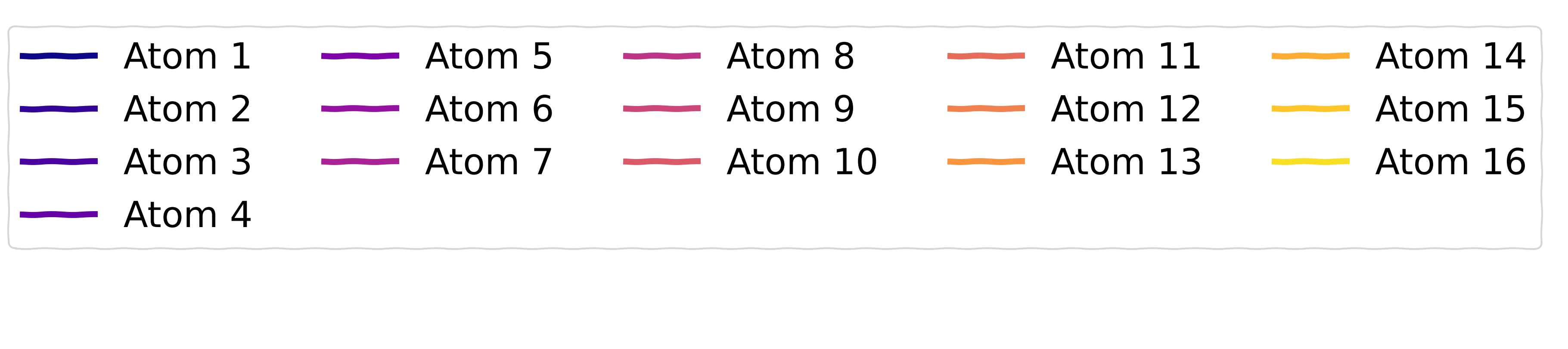
create_legend({'Atom %d'%(j+1): colors[j] for j in range(num_comps)}, params_leg = {'ncol': 5})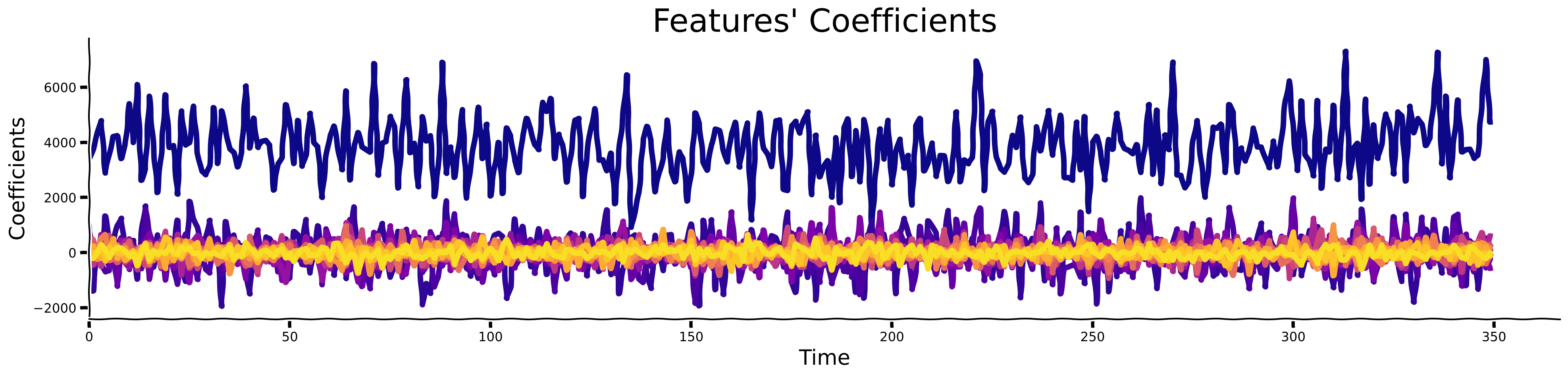
In this section, you’ve identified sparse components underlying natural images, similar to the approach taken by Olshausen and Field (1996) [2], which led to the widespread use of Dictionary Learning in research.
Interestingly, applying sparsity to the number of active components is crucial and closely related to how the visual cortex, including V1, processes visual information.
As discovered in seminal experiments by Hubel and Wiesel [mentioned before in 1], neurons in V1 are tuned to respond optimally to specific, sparse patterns of visual stimuli—this represents an efficient data representation that minimizes redundancy while maximizing information content.
This mechanism demonstrates that neurons in V1 intensely fire for certain edge orientations and light patterns, closely paralleling the sparse coding models used today in AI.
How do you think these insights about V1 might enhance the algorithms you will develop in the field of neuroAI?
What other neural mechanisms do you think utilize sparsity and can inspire AI research?
Summary
Estimated timing of tutorial: 1 hour 20 minutes.
In this tutorial, we first discovered the notion of “sparsity” by looking at the signal and its temporal difference. We also introduced kurtosis as one of the main metrics used to measure sparsity. We visually observed this effect by looking at the histograms of pixel values. Then, we introduced the notion of “sparse coding” by deriving fundamental units (basis) that constitute complex signals. For that, we used the OMP algorithm and compared the identified features to those found by applying PCA. In the end, we used the algorithm for 2 datasets: MNIST & CIFAR10.
The Big Picture
The main message we would like you to take away from this tutorial is that sparsity has numerous advantageous properties for representing computation in the brain and in AI models. We know the brain likely uses this principle extensively. The mechanisms to measure and induce sparsity in computational models of neuroscience and AI are important and we hope you have gained an idea of how you might think about applications of sparsity in the future.
In the next tutorial, we will look at another essential operation to be realized in brains & machines - normalization. If you have time at the end of this day’s tutorials, we have also included some further bonus material that covers the interesting application of spatial sparsity. If you’re running low on time, please concentrate on the other tutorials and come back to the bonus material at a more convenient time.